Open Journal of Marine Science
Vol.4 No.1(2014), Article ID:42525,11 pages DOI:10.4236/ojms.2014.41005
An Innovative and High-Speed Technology for Seawater Monitoring of Asinara Gulf (Sardinia-Italy)
1UTAGRI-ECO, ENEA, Roma, Italy
2InTReGA, Spin-Off ENEA, Sassari, Italy
3Department of Territorial Engineering, Geopedology and Applied Geology Section, University of Sassari, Sassari, Italy
4Department of Sciences for Nature and Environmental Resources, University of Sassari, Sassari, Italy
5UTAPRAD-DIM, ENEA, Frascati, Italy
Email: *maria.sighicelli@enea.it, Ileana.iocola@gmail.com, dpittalis@uniss.it, luglie@uniss.it, bmpadedda@uniss.it, pulinasi@uniss.it, Massimo.iannetta@enea.it, ivano.menicucci@enea.it, luca.fiorani@enea.it, antonio.palucci@enea.it
Copyright © 2014 Maria Sighicelli et al. This is an open access article distributed under the Creative Commons Attribution License, which permits unrestricted use, distribution, and reproduction in any medium, provided the original work is properly cited. In accordance of the Creative Commons Attribution License all Copyrights © 2014 are reserved for SCIRP and the owner of the intellectual property Maria Sighicelli et al. All Copyright © 2014 are guarded by law and by SCIRP as a guardian.
Received November 10, 2013; revised December 18, 2013; accepted December 30, 2013
KEYWORDS
Laser Excitation; Deconvolution; Chlorophyll-a; Algal Pigments; Environmental Monitoring
ABSTRACT
Laser induced fluorescence technique for sea water monitoring allows no-time consuming, non-invasive and non-destructive controls. In this study, the performance of the new shipboard laser spectrofluorometric CASPER (Compact and Advanced Laser Spectrometer—ENEA Patent) for monitoring phytoplankton community composition was examined. The prototype CASPER is based on double laser excitation of water samples in the UV (266 nm) and visible (405 nm) spectral region and a double water filtration in order to detect both quantitative data, such as chromophoric dissolved organic matter (CDOM), proteins-like components (tyrosine, tryptophan), algal pigments (chlorophylls a and b, phycoerythrin, phycocyanin, different pigments of the carotenoid groups) and qualitative data on the presence of hydrocarbons and oil pollutants. Sea water samples from different depths have been collected and analyzed from August 2010 through November 2011 in the Gulf of Asinara (N-W Sardinia). Several sampling stations were selected as sites with different degree of pollution. The accuracy and the reliability of data obtained by CASPER have been evaluated comparing the results with other standard measurements such as: Chlorophyll a (Chl a) data obtained by spectrophotometric method and total phytoplankton abundance in terms of density and class composition. Spectral deconvolution technique was developed and integrated with CASPER system to assess and characterize a marker pigments and organic compounds in situ and in vivo. Field studies confirmed CASPER system capability to effectively discriminate characteristic spectra of fluorescent water constituents, contributing to decrease the time-consuming manual analysis of the water samples in the laboratory.
1. Introduction
The oceans and coastal water quality assessment systems need to cover large areas with adequate spatial and temporal resolution. Furthermore, the operations must be cost-efficient and involve high-speed data processing. Such requirements are not easily met with traditional methods of water sampling and laboratory analysis and then additional information is necessary to detect and identify sources of water contamination, a critical water quality component.
Several critical components still remain missing or not adequately sampled to characterize the marine ecosystem biodiversity and habitat change [1].
Phytoplankton is an important biotic component and key biological quality element of the ecological status of water bodies, according to the Water Framework Directive (WFD) and the Marine Strategy [2]. It is a sensitive bio-indicator of ecosystem general health, its nutrient status, eutrophication, pollutants, and other anthropogenic impacts in aquatic environments [3]. As primary producer, it is capable of responding to changes in nutrient and toxin input, hydrology, sedimentation, irradiance and temperature regimes over a wide range of time scales. Phytoplankton can be subdivided into taxonomic groups (Chlorophytes, Cryptophytes, Cyanobacteria, Diatoms, and Dinoflagellates) that play important roles in coastal primary production, nutrient cycling, and food web dynamics. Numerous studies have shown that organic pollution or enhanced nutrient may cause changes on phytoplankton taxonomic composition and biomass [4,5]. In particular, it has been demonstrated that blooms of particular species or groups (for example Cyanophyceae, Dinophyceae) can indicate the occurrence of worse quality water [6,7].
The only reliable technique for identifying and enumerating phytoplankton species or groups is microscopy [8], a time-consuming and costly procedure that requires a high expertise level. Alternatively, phytoplankton biomass may be estimated from photopigment content.
Chlorophyll a measurements have been used for this purpose for many years, being considered as a first-level indirect indicator of ecosystem eutrophication.
Then, an extended set of phytoplankton characteristics, including their productivity, photosynthetic capacity, physiological status and taxonomic composition, needs to be monitored for improved ecosystem characterization. In recent years, the laser induced fluorescence (LIF) technique has been widely applied for water quality assessment in marine and freshwater environment. LIF technique allows no-time consuming, non-invasive and non-destructive sampling, without sample pre-treatment. It is based on the measurements of the laser-induced water emission to retrieve qualitative and quantitative information about the in situ fluorescent constituents [9]. In vivo fluorescence of Chlorophyll a and accessory pigments (chlorophylls b/c, phycobiliproteins and carotenoids) is generally used as an index of Chlorophyll a concentration and phytoplankton biomass [10,11] and offers useful information for structural and phytophysiological characterization of the mixed algal populations [9,12-14].
Besides the broadband chromophoric dissolved organic matter (CDOM), fluorescence emission can be used for assessment of CDOM abundance and its qualitative characterization [9,15].
However, many commercially field fluorometers employ spectrally broad fluorescence but do not yield an adequate excitation and spectral resolution to assure reliable estimate of the fluorescent constituents in spectrally complex natural waters. This spectral complexity leads to many interpretation problems of the fluorescence measurements and compromises the fluorescence assessments accuracy. To address this issue, recent studies revealed that it is essential to develop spectral deconvolution analysis of the LIF signatures to retrieve information from overlapped spectral patterns of aquatic fluorescent constituents [9].
The aim of the present work was to investigate the performance of the new portable laser apparatus CASPER (Compact and Advanced laser SPE ctrofotometeR —ENEA Patent) for phytoplankton pigments composition analysis, oil derivates detection and seawater quality monitoring in the Gulf of Asinara (N-W Sardinia).
The northern coast of Sardinia is one of the most dynamic and vulnerable environments in the Western Mediterranean. It includes the Asinara Island National Park, a part of the “Sanctuary of the Cetaceans” of the Mediterranean Sea and well known beautiful tourist place. Important civil and industrial activities (harbours, power and chemical plants) coexist with these high naturalistic quality aspects.
CASPER attempts to improve measurements of chlorophylls and accessory pigments and organic compounds contributing to assess phytoplankton physiological/nutrient status, and to provide basic structural characterization of phytoplankton community, assessment of CDOM and water turbidity. These variables offer valuable, currently missing information for improved bio-environmental characterization of coastal aquatic ecosystems.
In this work, we describe a fluorescence spectral system to detect and assess water fluorescence compounds by means of a spectral deconvolution technique, based on laboratory and field measurements and implemented in open source R software environment (http://www.rproject.org/), in order to contribute to identify marker pigments and phytoplankton groups using the discriminatory capability of characteristic spectra recorded by CASPER.
2. Material and Methods
2.1. Study Site and Field Sampling
Field studies for water quality assessment of Gulf of Asinara were conducted from August 2010 to November 2011. Sea water samples from 0 to 10 m depth were collected and analysed by CASPER.
The stations were situated along six transects perpendicular to the coastline, respectively from more impacted areas to less ones, from the town of Porto Torres in the central part of the gulf to Cala Reale in the Asinara Island (Figure 1(a), red points).
Each transect comprises three stations at 500, 1500
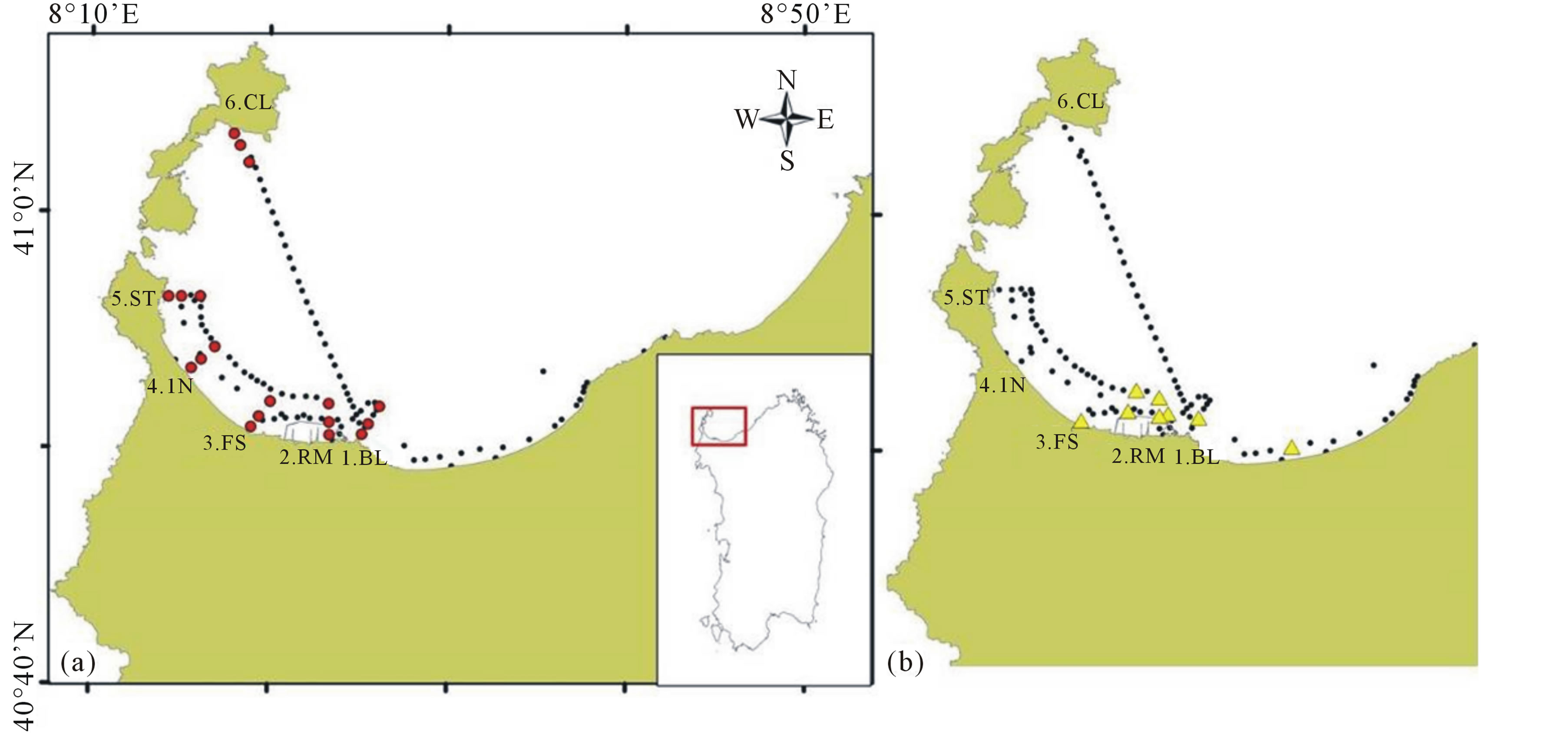
Figure 1. (a) Sampling stations in the Gulf of Asinara (Sardinia): red points indicate the stations along the selected six transects (1. BL-Balai; 2. RM-Rio Mannu; 3. FS-Fiume Santo; 4. IN-Intermedio; 5. ST-Stintino; 6. CL-Cala Reale), the black points indicate the tracks of the raft cruises; (b) Stations (in yellow) where pollutants were found during the field sampling.
and 3000 m from the coast. Periodic raft cruises were also conducted in gulf to extend the sampling area to collect more data useful for the validation of remote sensing algorithms (Figure 1(a), black points).
Samples along transects were collected on 3/08/2010, 16/12/2010, 29/04/2011 and 30/11/2011, while cruises were conducted on 9/02/2011, 8/07/2011 and 14/11/2011.
Water samples for chemical analyses were collected and preserved in cold, dark conditions for laboratory analyses of alkalinity, ammonia (NH4), nitrate (NO3), nitrite (NO2), reactive silica (RSi), orthophosphate (RP) and total phosphorus (TP), following Strickland & Parsons (1972) [16] and Scor-Unesco (1997) [17] for Chl a (data not shown).
Dissolved inorganic nitrogen (DIN) was obtained as the sum of ammonia, nitrate and nitrite. Temperature, salinity, dissolved oxygen (DO), pH and fluorimetric Chlorophyll a (fChl a) were measured in situ with a multi-parameter probe (YSI model 6600 V2).
On 11 January 2011, an accident occurred in the Asinara Gulf during fuel uploading operations of Fiume Santo power plant in the Porto Torres industrial area, causing heavy fuel oil loss (about 50 tons) into the sea. The stations where potential pollutants were found and collected during the samplings were principally located in industrial area of the gulf (Figure 1(b)).
2.2. Phytoplankton Analysis
In the nearer coastline stations of transects BL, FS, ST and CL (Figure 1(a)) superficial water samples were collected to assess phytoplankton species composition, total cell densities and physical-chemical parameters. Phytoplankton samples were fixed with Lugol’s solution and analysed according to Utermöhl technique [8], using an inverted microscope (Zeiss, Axiovert 25) after the sedimentation of 100 cm3 of water. Cell counts were made at 100× on the entire bottom of the sedimentation chamber for the larger and more easily identifiable species, and replicated at 200× and 400× on an adequate number of fields for the smaller cells. Species were determined using traditional phycological determination manuals [18-27]. Unidentified cells of size < 20 μm were considered in the dimensional group of nanoplankton.
2.3. Compact and Advanced Laser SPEctrofotometeR (CASPER)
Figure 2(a) shows the picture of CASPER. Based on LIF technique to record spectra of the water samples, the instrument is equipped with two lasers, ultraviolet (UV) laser (excitation wavelength, λex: 266 nm) and blue (BL) laser (λex: 405 nm). Its operation scheme is explained in the block diagram of flow-through system (Figure 2(b)).
Water flow, pushed in the pipes by one pumping unit (not shown) and two valves (not shown), permit to fill quartz cuvettes (C1 and C2). To properly characterize seawater bio-optical features, water sample constituents are selectively filtered first to arrive in the cuvette C2 with a 0.22 μm porosity filter that ensures to pass only dissolved matters. Each laser beam is alternatively activated by respective shutter (not shown) and directed through the collimating lens to cuvettes. LIF emission signal output from each cuvette is collected and coupled by a fiber optic to an Ocean Optics spectrometer for spectral analysis in the 200 - 800 nm range. Typical sample measurement cycle requests a few minutes and involves

Figure 2. Compact and advanced laser SPEctrofluorometeR (Casper): picture of the instrument (a) and block diagram (b).
the recording of four spectra: two spectra for every laser in each cuvette, BL1-BL2 and UV1-UV2.
CASPER has been devised for field campaigns, for this it is battery operated and fully controlled by a portable computer. Operational software developed in Visual Basic activates the instrument by an ad hoc microcontroller electronic module and controls all instrumental settings. Instead, Ocean Optics software tools through the USB ports connected to PC control the two spectrometers.
2.4. Casper Analysis and Data Processing
Recently CASPER has engaged in several measurements campaigns, monitoring diverse water types (Arctic Ocean, Mediterranean Sea and numerous estuaries and rivers in Italy, Canada and other European countries). In previous works, the data retrieved from the spectral signatures have been used to supply valuable qualitative information for the investigated water body and only few compounds (like Chl a) were transformed in quantitative values [28-31]. In this study spectral deconvolution analysis has been developed and combined with the laboratory and field fluorescence measurements to identify different aquatic constituents and retrieve correct individual spectral bands for water sample assessment.
The LIF emission spectra recorded by CASPER are the result of the overlapping spectra of the individual compounds excited by the laser beam. The spectral deconvolution analysis performed on CASPER LIF spectra consists of linear amplitude scaling of the basic spectral components to provide the best fit of the spectrum resulting from their summation to the LIF signature in the selected spectral range.
LIF signal can be modeled by a combination of single Gaussian peak corresponding to the emission of each component present in the water sample characterized by amplitude, position and width.
Only signals recorded in C1 in C2, respectively excited by visible laser (BL1) and by ultraviolet laser (UV2), were examined (Figure 3) through the deconvolution protocol to detect pigments content and dissolved substances. A list of basic spectral components included in the deconvolution procedure for BL1 and UV2 to explain the LIF spectral variability observed in field is reported in Table 1. The set of spectral components used in this study was identified and gathered from single spectra of SIGMA-Aldrich reference samples measured in laboratory obtaining peak positions and variances.
Peak positions of the most representative pigments were compared with those reported in the literature. Few works [32,33] show emission bands of fucoxanthin corresponding to wavelengths near our laboratory measurement (around 665 nm). In literature, some spectral signatures of cyanobacterial, containing allophycocyanin, have shown emission peaks around 662 nm [34,35]. Emissions at 662 - 665 nm were also reported for signatures of senescent phytoplankton cultures, consistently with the presumable photodegradation origin of the emission [9].
A code written in R software environment was used to process fluorescence signals recorded by CASPER and carry out the automatic spectral deconvolution procedure through a series steps. The results elaborated by code are stored in ASCII data files and graphic outputs. First step is a subtraction of the electronic and light backgrounds from the fluorescence spectrum and correction of spectrometer radiometric values through standard spectra and then application of Savitzky-Golay smoothing filter to render visible the relative widths and heights of spectral lines in noisy spectrometric data.
Using the R function nls through the weighted summation of the spectral components listed in Table 1, it is achieved the best fit of the measured spectrum. Fitting does not modify either band centre or width of each

Figure 3. Gaussian deconvolutions of surface water sample in C1 excited at 405 nm (BL1) and in C2 excited by 266 nm (UV2). The sample was collected in FS station at 1500 m from coast in February 2011.

Table 1. Spectral components used for LIF signals deconvolution of water samples in C1 excited at 405 nm (BL1) and in C2 excited by 266 nm (UV2).
component. Only amplitudes of peaks can be finely tuned by the program. The magnitudes of these coefficients are automatically varied until the sum of squares of residuals between modeled and measured signal is minimized.
The fitting procedure is applied only in spectral range from 420 to 700 nm for BL1 and from 250 to 700 nm for UV2, where the emission peaks of the key aquatic constituents are located.
The four processed signals (BL1, BL2, UV1, UV2) and intensities obtained by the multiple Gaussian deconvolution are normalized to the related water Raman peak for releasing data in Raman units (RU). The latter units are generally adopted in order to correlate measurements performed on same water samples using different local or remote instruments and to compare different water samples [36].
The most of the constituents LIF intensities has been converted in concentration units through a series of laboratory and field calibrations. SIGMA-Aldrich reference samples reported in Table 2 were purchased and used to detect and calibrate the water compounds emission peaks.
3. Results and Discussion
3.1. Laboratory Measurements
Temporal and spatial phytoplankton class composition in terms of density percentage is reported in Figure 4. Bacillariophyceae, Dinophyceae and Cryptophyceae dominated phytoplankton composition in each sampling period with smaller and varying contributions of Cyanophyceae and green algae (Chlorophyceae, Euglenophyceae and Prasinophyceae). The Bacillariophyceae were mainly represented by Leptocylindrus minimus Gran (11 × 103 cell∙l−1 in August 2010 at ST) and Leptocylindrus danicus Cleve (12 × 103 cell∙l−1 in December 2010 at FS and 11 × 103cell∙l−1 in April 2011 at FS).
The Dinophyceae were mainly represented by Gyrodinium sp. (1.2 × 10³ cell∙l−1 in August 2010 at CL and 1.1 × 10³ cell∙l−1 in April 2011 at FS), and the Cryptophyceae were constituted principally by Plagioselmis sp. (32 × 103 cell∙l−1 in August 2010 at FS).
For Cyanophyceae the highest density value was observed in November 2011 at CL with Microcystis sp. (30 × 103 cell∙l−1).

Figure 4. Temporal and spatial phytoplankton class composition in terms of density percentage.
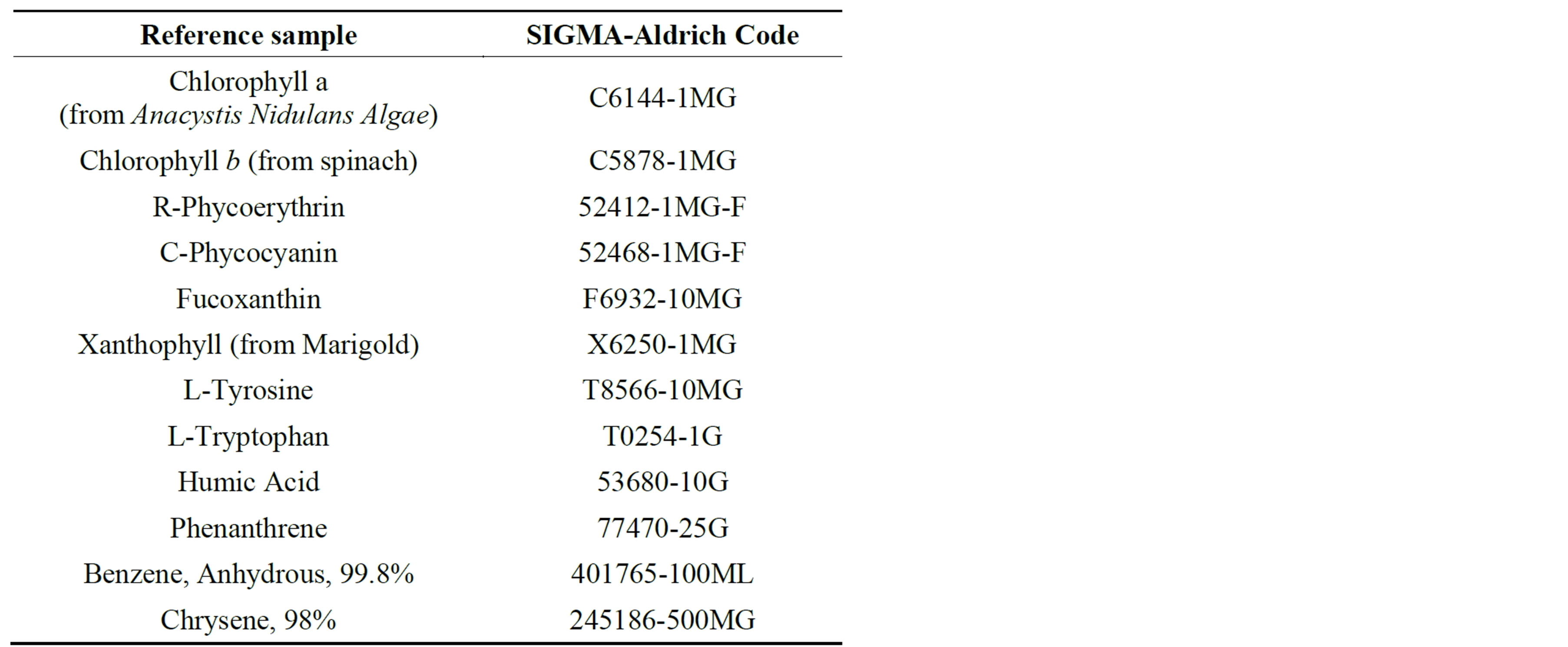
Table 2. List of the purchased reference samples.
3.2. Correlation Analysis
To evaluate CASPER capabilities of fluorescent constituents quantitative assessment, R.U. intensities values obtained by the instrument for Chl a at 682 nm were compared to Chl a spectrophotometric measurements. The Chl a CASPER intensities showed high correlation with spectrophotometric analysis (R2 = 0.9087) confirming the validity of CASPER LIF method to determine phytoplankton biomass (Figure 5).
To retrieve taxonomic information from spectral fluorescence analysis, the most important phytoplankton classes were divided in four spectral algal groups identified by microscopy analysis and characterized by similar fluorescence excitation spectra resulting from composition of chlorophylls and accessory pigments [14]:
• The Green group (including Chlorophyceae, Euglenophyceae and Prasinophyceae) containing Chl a, Chl b and xanthophyll;
• The Blue group (Cyanophyceae) with phycobilisomes that function as peripheral antennae (mainly phycocyanin);
• The Brown group (Bacillariophyceae, Dinophyceae

Figure 5. Correlation between Chl a CASPER intensities and spectrophotometric analysis.
and Chrysophyceae) contain Chl a, Chl c and xanthophyll (often fucoxanthin or peridinin);
• The Mixed group (Cryptophyceae) that presents a combination of Chl a and Chl c with one phycobiliprotein that can be either phycoerythrin or phycocyanin.
The spectrofluorometric and phytoplankton microscopic evaluation have been compared and rendered in a correlation matrix (Table 3) using Pearson coefficient (r). The matrix was realized using in x-axis the intensities obtained by Gaussian deconvolution process in Raman Units for peaks E_475, Tyr, E_330, Trypt, Total CDOM (given by the sum of humic and fulvic components), Chla and the indexes of phytoplankton (ratio potential algae-related R.U. intensities to R.U. Chl a intensities) for peaks XA, FE, E_615, FC, Chl b and FX.
In y-axis laboratory data were used: Chl a values, Brown, Green, Blue, Mixed densities (values in cell∙l−1), densities given by sum of the four groups (4 Groups Density) and total densities measured in each stations considering also taxa absent in previous groups. The peculiar peaks for each group are underscored and reported in cursive.
The correlation between Chl a measured by the spectrophotometer (Laboratory Chl a) vs. Chl a measured by

Table 3. Correlation matrix (Pearson coefficient) between CASPER and laboratory measurements. The peculiar peaks for each group are reported in red.
the spectrofluorometer (Chl a), is very high (r = 0.95) in according to previously shown in Figure 5. Laboratory Chl a has also shown a good correlation with peak at 475 nm (r = 0.80). Emission peak at 475 nm is mainly ascribed to suspended organic matter content (particulate included algae) and this can explain also the quite high correlation between E_475 vs. phytoplankton densities and vs. dominant algae groups (Mixed and Brown).
Moreover laboratory Chl a is positively correlated to tryptophan amino acid (r = 0.86). High values of correlation are also evident between tryptophan vs. total phytoplankton densities (r = 0.51) and Mixed groups (r = 0.66). Tryptophan and tyrosine are amino acids generally originated from proteins in dissolved organic matter released by recent biological activity (fecal pellets), bacteria exudates and degradation products of algae. Consequently exudates and degradation products of the algae may lead to an increased signal in the protein-like fluorescence [37].
A lower correlation of laboratory Chl a vs. Total CDOM (r = 0.27) confirms that we are in a coastal zone, also called Case II water [38].
Chl b pigments and carotenoids can potentially individuate Green algae group. In our matrix, Green group does not appear directly correlated to Chl b (r = 0.01), but it is important to note that Chl b have shown a positive value only for this group. The unexpected very low correlation can be understood taking into account both the poor density of this group in the phytoplankton composition and differences in the algae morphology: namely the presence of colonial algae can be responsible for an underassessment of Chl b concentration [39]. The nonphotosynthetic (photoprotective) carotenoids are distributed across taxa of Green group, but do not contribute to the excitation spectra [40].
Another unexpected result for Green group is the quite correlation with phycoerythrin peak (r = 0.38).
• In Blue groups the only positive correlation is vs. phycocianin (r = 0.29), the characteristic pigment of the class. For Cyanophyceae, as well as for the other groups with low densities in sampling (Green Group), a negative correlation with Chl a was found.
In addition, for cyanobacteria, most of the Chl a (80% - 90%) is located in the non-fluorescing photosystem I (PSI), and consequently a specific feature for Cyanobacteria is a very low Chl a in vivo fluorescence [41].
The Brown group have shown a relatively high correlation vs. Chl a (r = 0.42) as the Mixed group (r = 0.57). A very poor value is present for fucoxanthin band confirming current doubts for this peak.
The emission spectra for Cryptophyta (Mixed group) generally differ for those of other groups having a marked peak around 580 nm due to the presence of phycobilins, in particular phycoerithrin. A lower correlation with this peak (r = 0.19) in relation to the other bands has been found. A more high value was instead found for phycocyanin (r = 0.24). The Mixed algae can in fact have either phycoerithrin or phycocyanin as main accessory pigment. For this group it was found that the species-specific identification is available just for the first sampling, in which is present only Plagioselmis sp., that have phycoerithrin as major accessory pigment. In the other samples density data are sorted as undetermined Cryptophyceae.
To provide additional information about pertinent complex bio-geochemical processes in the water environments further investigation are necessary to interpret the origin of undefined bands emissions (at 550, 615 and 330 nm) and introduce in the deconvolution process the contributions of other diagnostic substances such as Chl c, peridin (characteristics of dinoflagellates) and alloxanthin (characteristics of Crytpophyceae) for a better individuation of algae groups.
3.3. Qualitative Detection of Hydrocarbons
The CASPER spectral analysis for determination of organic compounds in marine environment was applied on contaminated sea water samples.
In Figure 6, the comparison between fluorescence spectra of heavy fuel oil samples and CDOM shows the CASPER discriminatory capability of qualitative pollutants detection.
The oil has shown a peak emission at 450 - 500 nm. The fluorescence of naturally CDOM in the water interferes with the oil fluorescence signal [42,43]. In fact the fluorescence spectra excited at 266 nm for CDOM (humic-like component) and heavy oil are very similar in shape, width and spectra location. CASPER has proved to be a valid instrument to differentiate the two substances thanks to the filtration system that allows passage only to CDOM in the filtered cuvette C2.
Figure 7 shows fluorescence spectra of light oil (diesel) and some Polycyclic Aromatic Hydrocarbons (PAHs) purchased by SIGMA-Aldrich. PAHs are a class of organic compounds formed during incomplete combustion or pyrolysis of organic matter occurring in a variety of natural processes or human activities.
These pollutants can enter in the sea water by means routes, including petroleum spill, runoff from roads, sewage, effluents from industrial processes, and fallout from the atmosphere [44].
Examined pollutants have shown peaks at lower wavelengths around 350 - 400 nm. Moreover, also in these cases, they present an important reduction of emission intensities in 0.22 μm filtered cuvette (Figure 7). For this reason it is possible to detect the presence of oil pollution or PAHs just observing emission spectra differences in range 350 - 400 nm or 450 - 500 nm of cuvettes excited by UV laser without (C1-UV1) and with filtration (C2- UV2)
4. Conclusions
The laser induced fluorescence spectra of marker pigments and groups remains one of the successful bio-optical techniques for the differentiation of phytoplankton groups in vivo and in situ.
Both laboratory and field CASPER measurements without sample pre-treatment suggest that CASPER is a useful tool to provide the reliable data of Chl a concentrations and taxonomic information of dominant algal groups.
Obviously, microscopy and laboratory analysis are required and necessary for higher taxonomical levels identification of phytoplankton species, but CASPER can supply a rapid diagnostic and early warning system to detect algal blooms and contribute to assess the eutrophic status of water bodies.

Figure 6. Fluorescence spectra (in Raman units) of CDOM (upper) and heavy oil (bottom) diluted in MilliQ water and excited at 266nm without (left, C1) and after filtration (right, C2).

Figure 7. Fluorescence spectra (in Raman units) of the following substances: (a) Diesel; (b) Chrysene; (c) Phenanthrene; (d) Benzene; diluted in MilliQ water and excited at 266 nm before (C1) and after filtration (C2).
In most cases, the recorded signatures measured in the Asinara Gulf are relatively simples and mostly determined by the overlapped spectral bands of organic matter and Chl a fluorescence (with the fits almost indistinguishable from the measured spectra).
Nevertheless, CASPER needs more robust and suitable algorithms to describe the asymmetrical spectral shape of the emission bands to ensure reliable assessment of the fluorescent constituents in spectrally complex natural waters.
Work still needs to be done to fully implement the analytical potential of the CASPER system.
In particular, most of the constituent fluorescence parameters obtained by suitable algorithms need to be correlated with independent algal pigment concentration measurements (e.g. data analysis by HPLC) and the robustness of the correlation must to be verified in an extended concentration range considering also seasonal variability.
Hence, starting from a good relationships found between Chl a fluorescence retrievals and independent measurements of Chl a content and analysing also peak asymmetry through spectral deconvolution will be possible develop analytical algorithms to improve biomarker pigments assessment and phytoplankton assemblage.
At the moment, field measurements and spectral analysis highlight the utility of the CASPER analytical system as an informative integrated tool for water research and environmental monitoring.
Acknowledgements
This work was funded by Autonomous Region of Sardinia, PO Sardegna FSE 2007-2013 L.R. 7/2007 “Promotion of Scientific Research and Innovative Technologies in Sardinia”. The authors are thankful to the Technical Office of the Parco Nazionale dell’Asinara for providing the scientific permits.
REFERENCES
- A. M. Chekalyuk, K. A. Moore, D. L. White and D. E. Porter, “Advanced Laser Fluorescence (ALF) Technology for Estuarine and Coastal Environmental Bio-Monitoring,” 2006. http://ciceet.unh.edu/briefs/charette_brief/chekalyuk_final.pdf
- European Parliament and Council, “Water Framework Directive,” Directive 2000/60/EC, 2000, pp. 1-73.
- A. B. Barbosa, R. B. Domingues and H. M. Galvão, “Environmental Forcing of Phytoplankton in a Mediterranean Estuary (Guadiana Estuary. South-Western Iberia): A Decadal Study of Anthropogenic and Climatic Influences,” Estuaries and Coasts, Vol. 33, No. 2, 2010, pp. 324-341. http://dx.doi.org/10.1007/s12237-009-9200-x
- P. M. Glibert, C. E. Wazniak, M. R. Hall and B. Sturgis, “Seasonal and Interannual Trends in Nitrogen and Brown Tide in Maryland’s Coastal Bays,” Ecological Applications, Vol. 17, No. 5, 2007, pp. 79-87. http://dx.doi.org/10.1890/05-1614.1
- G. M. Hallegraeff, “Ocean Climate Change. Phytoplankton Community Responses and Harmful Algal Blooms: A Formidable Predictive Challenge,” Journal of Phycology, Vol. 46, No. 2, 2010, pp. 220-235. http://dx.doi.org/10.1111/j.1529-8817.2010.00815.x
- K. Sivonen and G. Jones. “Cyanobacterial Toxins,” In: I. Chorus, J. Bartram, Eds., Toxic Cyanobacteria in Water: A Guide to Public Health Significance, Monitoring and Management, E & FN Spon, London, 1999, pp. 41-111.
- H. Kaas and P. Henriksen, “Saxitoxins (PSP Toxins) in Danish Lakes,” Water Research, Vol. 34, No. 7, 2000, pp. 2089-2097. http://dx.doi.org/10.1016/S0043-1354(99)00372-3
- H. Utermöhl, “Zur Vervollkommnung der Quantitative Phytoplankton-Methodik,” Mitteilungen Internationale Vereins Theoretisch Angewiesen Limnologie, Vol. 9, 1958, pp. 1-38.
- A. M. Chekalyuk and M. Hafez, “Advanced Laser Fluorometry of Natural Aquatic Environments,” Limnology and Oceanography Methods, Vol. 6, 2008, pp. 591-609. http://cce.lternet.edu/docs/bibliography/Public/063ccelter.pdf http://dx.doi.org/10.4319/lom.2008.6.591
- Z. Kolber and P. G. Falkowski, “Use of Active Fluorescence to Estimate Phytoplankton Photosynthesis in Situ,” Limnology and Oceanography, Vol. 38, No. 3, 1993, pp. 1646-1665. http://dx.doi.org/10.4319/lo.1993.38.8.1646
- M. K. H. Beutler, K. H. Wiltshire, B. Meyer, C. Moldaenke and H. Dau, “In Situ Profiles of Phytoplankton: Algal Composition and Biomass Determined Fluorometrically,” In: G. Hallegraeff, S. I. Blackburn, C. J. Bolch and R. J. Lewis, Eds., Harmful Algal Blooms 2000 Proceedings Volume, Intergovernmental Oceanographic Commission of UNESCO, Paris, 2001, pp. 202-205.
- C. S. Yentsch and C. M. Yentsch, “Fluorescence Spectral Signatures-Characterization of Phytoplankton Populations by the Use of Excitation and Emission Spectra,” Journal of Marine Research, Vol. 37, No. 3, 1979, pp. 471-483.
- L. Poryvkina, S. Babichenko, S. Kaitala, H. Kuosa and A. Shalapjonok, “Spectral Fluorescence Signatures in the Characterization of Phytoplankton Community Composition,” Journal of Plankton Research, Vol. 16, No. 10, 1994, pp. 1315-1327. http://dx.doi.org/10.1093/plankt/16.10.1315
- M. K. H. Beutler, K. H. Wiltshire, B. Meyer, C. Moldaenke, C. Luring, M. Meyerhofer, U. P. Hansen and H. Dau, “A Fluorometric Method for the Differentiation of Algal Populations in Vivo and in Situ,” Photosynthesis Research, Vol. 72, No. 1, 2002, pp. 39-53. http://dx.doi.org/10.1023/A:1016026607048
- N. Hudson, A. Baker and D. Reynolds, “Fluorescence Analysis of Dissolved Organic Matter in Natural Waste and Polluted Waters—A Review,” River Research and Applications, Vol. 23, No. 6, 2007, pp. 631-649. http://dx.doi.org/10.1002/rra.1005
- J. D. H. Strickland and T. R. Parsons, “A Manual of Seawater Analysis,” 2nd Edition, Fisheries Research Board of Canada, Bulletin 167, 1972.
- SCOR-UNESCO, “Determination of Photosynthetic Pigments in Sea Water,” UNESCO Monographs on Oceanographic Methodology, Paris, 1997.
- E. E. Cupp, “Marine Plankton Diatoms of the West Coast of North America,” Otto Koeltz Science Publishers, Koenigstein W, Germany, 1977.
- L. Rampi and R. Bernhard, “Key for the Determination of Mediterranean Pelagic Diatoms,” Comitato Nazionale Energia Nucleare RT/BIO 78-1, Roma, 1978.
- L. Rampi and R. Bernhard, “Chiave per la Determinazione Delle Peridinee Pelagiche Mediterranee,” Comitato Nazionale Energia Nucleare RT/B10 80-8, Roma, 1980.
- H. J. Humm and S. R. Wicks, “Introduction and Guide to the Marine Blue-Green Algae,” John Wiley & Sons Inc., New York, 1980.
- H. Germain, “Flore des Diatomèes Eaux Douces et Saumatres,” Ed. Boubée, Paris, 1981.
- L. Rampi and M. Bernhard, “Chiave per la Determinazione Delle Peridinee Pelagiche Mediterranee,” Comitato Nazionale Energia Nucleare RT/BIO 81-13, Roma, 1981.
- F. Husted, “The Pennate Diatoms,” Koeltz Scientific Books, Koenigstein, 1985.
- A. Sournia, “Atlas du Phytoplancton Marin. Volume I: Introduction. Cyanophycées. Dictyochophycées. Dinophycées et Raphidophycées,” Editions CNRS, Paris, 1986.
- M. Ricard, “Atlas du Phytoplancton Marin. Volume II: Diatomophycées,” Editions CNRS, Paris, 1987.
- C. R. Tomas, “Identifying Marine Phytoplankton,” Academic Press, New York, 1997.
- P. Aristipini, D. Del Bugaro, L. Fiorani, S. Loreti and A. Palucci, “Mobile Laser Spectrofluorometer for Natural Waters Monitoring in Sicily,” Proceedings of SPIE, Advanced Laser Technologies 2004, Dresden, 2005, pp. 190- 195. http://dx.doi.org/10.1117/12.633542
- D. Caputo-Rapti, L. Fiorani and A. Palucci, “Compact Laser Spectrofluorometer for Water Monitoring Campaigns of Southern Italian Regions Affected by Salinization and Desertification Processes,” Journal of Optoelectronics and Advanced Materials, Vol. 10, No. 2, 2008, pp. 461-469.
- F. Colao, R. Fantoni, L. Fiorani, V. Lazic, A. Palucci, E. Demetrio and I. Okladnikov, “Dissolved and Particulate Organic Matter Measured with the ENEA Portable Laser Fluorometer during the 2006 Polish Summer Oceanographic Arctic Campaign (Svalbard Islands),” Technical Reports of the Italian Agency for New Technologies Energy and the Environment, Rome, 2008.
- M. Cisek, F. Colao, E. Demetrio, A. Di Cicco, V. Drozdowska, L. Fiorani, I. Goszczko, V. Lazic, I. Okladnikov, A. Palucci, J. Piechura, C. Poggi, M. Sighicelli, W. Walczowski and P. Wieczorek, “Remote and Local Monitoring of Dissolved and Suspended Fluorescent Organic Matter off the Svalbard,” Journal of Optoelectronics and Advanced Material, Vol. 12, No. 7, 2010, pp. 1604-1618.
- K. Tetzuya, N. Umpei and M. Mamoru, “Fluorescence Properties of the Allenic Carotenoid Fucoxanthin: Implication for Energy Transfer in Photosynthetic Pigment Systems,” Photosynthesis Research, Vol. 27, No. 3, 1991. pp. 221-226.
- E. Papagiannakis, I. H. M. van Stokkum, H. Fey, C. Buchel and R. van Grondelle, “Spectroscopic Characterization of the Excitation Energy Transfer in the Fucoxanthin-Chlorophyll Protein of Diatoms,” Photosynthesis Research, Vol. 86, No. 1, 2005, pp. 241-250. http://dx.doi.org/10.1007/s11120-005-1003-8
- C. O. Heocha, “Biliproteins of Algae,” Annual Review of Plant Physiology, Vol. 16, No. 1, 1965, pp. 415-434. http://dx.doi.org/10.1146/annurev.pp.16.060165.002215
- A. M. Wood, P. K. Horan, K. Muirhead, D. Phinney, C. M. Yentsch and J. B Waterbury, “Discrimination between Types of Pigments in Marine Synechococcus spp. by Scanning Spectroscopy, Epifluorescence Microscopy and Flowcytometry,” Limnology and Oceanography, Vol. 30, No. 6, 1985, pp. 1303-1315. http://dx.doi.org/10.4319/lo.1985.30.6.1303
- S. Determann, R. Reuter, P. Wagner and R. Willkomm, “Fluorescent Matter in the Eastern Atlantic Ocean. Part 1: Method of Measurement and Near-Surface Distribution,” Deep Sea Research Part I: Oceanographic Research Papers, Vol. 41, No. 4, 1994, pp. 659-675. http://dx.doi.org/10.1016/0967-0637(94)90048-5
- S. Determann, J. M. Lobbes, R. Reuter and J. Rullkotterb, “Ultraviolet Fluorescence Excitation and Emission Spectroscopy of Marine Algae and Bacteria,” Marine Chemistry, Vol. 62, No. 1, 1998, pp. 137-156. http://dx.doi.org/10.1016/S0304-4203(98)00026-7
- A. Morel and L. Prieur, “Analysis of Variations in Ocean Color,” Limnology and Oceanography, Vol. 22, No. 4, 1977, pp. 709-722. http://dx.doi.org/10.4319/lo.1977.22.4.0709
- A. Lai, P. Giordano, R. Barbini, R. Fantoni, S. Ribezzo and A. Palucci, “Bio-Optical Investigation on the Albano Lake,” Proceedings of EARSeL-SIG-Workshop LIDAR, Dresden, 2000, pp. 185-195.
- G. Johnsen and E. Sakshaug. “Bio-Optical Characteristics of PSII and PSI in 33 Species (13 Pigment Groups) of Marine Phytoplankton and the Relevance for Pulse-Amplitude-Modulated and Fast Repetition-Rate Fluorometry,” Journal of Phycology, Vol. 43, No. 6, 2007, pp. 1236- 1251. http://dx.doi.org/10.1111/j.1529-8817.2007.00422.x
- D. Campbell, V. Hurry, A. K. Clarke, P. Gustafsson and G. Öquist, “Chlorophyll Fluorescence Analysis of Cyanobacterial Photosynthesis and Acclimation,” Microbiology and Molecular Biology Reviews, Vol. 62, No. 3, 1998, pp. 667-683.
- S. V. Patsayeva, “Fluorescent Remote Diagnostics of Oil Pollutions: Oil in Films and Oil Dispersed in the Water Body,” EARSel Advances in Remote Sensing, Vol. 3, No. 3-VII, 1995, pp. 170-178.
- A. G. Ryder, “Analysis of Crude Petroleum Oils Using Fluorescence Spectroscopy,” Reviews in Fluorescence, Vol. 2005, 2005, pp. 169-198. http://dx.doi.org/10.1007/0-387-23690-2_8
- J. J. Santana Rodriguez and C. Padron Sanz, “Fluorescence Techniques for Determination of Polycyclic Aromatic Hydrocarbons in Marine Environment: An Overview,” Luminescence Spectroscopy, Analusis, Vol. 28, No. 8, 2000, pp. 710-717. http://dx.doi.org/10.1051/analusis:2000280710
NOTES
*Corresponding author.