American Journal of Industrial and Business Management
Vol. 2 No. 2 (2012) , Article ID: 18843 , 8 pages DOI:10.4236/ajibm.2012.22007
A Batch Arrival Queue System with Coxian-2 Server Vacations and Admissibility Restricted
![]()
Department of Statistics, Allameh Tabataba’i University, Tehran, Iran.
Email: badamchi@yahoo.com
Received October 22nd, 2011; revised December 18th, 2011; accepted January 4th, 2012
Keywords: Mx/G/1 Queue; Restricted Admissibility Policy; Bernoulli Vacation; Optional Vacation; Mean Queue Size; Mean Response Time
ABSTRACT
The M/G/1 classic queueing system were extended by many authors in last two decades. The systems with server’s vacation are important models that extend the M/G/1 queueing system. Also another conditions such as admissibility restricted may occure in systems. From this motivation, in this system I consider a single server queue with batch arrival Poisson input. There is a restricted admissibility of arriving batches in which not all batches are allowed to join the system at all times. At each service completion epoch, the server may apt to take a vacation with probability θ or else with probability 1 − θ may continue to be available in the system for the next service. The vacation period of the server has two heterogenous phases. Phase one is compulsory, and phase two follows the phase one vacation in such a way that the server may take phase two with probability p or may return back to the system with probability 1 − p. The vacation times are assumed to be general. All stochastic processes involved in this system (service and vacation times) are independent of each other. We derive the PGF’s of the system and by using them the informance measures are obtained. Some numerical approaches are examined the validity of results.
1. Introduction
The concept of vacation in the M/G/1 queueing system were studied by Keilson and Servi in [1]. They introduced the concept of modified service time which has a main rule in the systems with general service and vacation times.
In many examples such as production system, bank services, computer and communication networks; the system have vacation. For overhauling or maintenance the system the server may go to vacation.
For the systems with batch arrival the vacation time were analyzed by Baba in [2], he derived the queue size distribution, waiting time distribution and busy period distribution of Mx/G/1 queue with vacation times using the well known supplementary variable technique.
In many systems with batch arrival there is a restriction such that not all batches are allowed to join the system at all time. This policy is named restricted admissibility. For the first time Madan and Abu-Dayyeh [3,4] proposed an Mx/G/1 queueing system with restricted admissibilty of arriving batches and Bernoulli schedule server vacation. Alnowibet and Tadj [5], also Madan and Choudhury [6] and Choudhury [7] work on this concepts.
Recently author in [8] studied a batch arrival queueing system with two phases of heterogenous service with optional second service and restricted admissibility with single vacation policy.
In fact this paper is a generalization of [9] in which the authors inspected a M/G/1 system with coxian-2 server vacation.
This paper adresses issue of model building of manufacturing systems of job-shop type, where the server takes vacations after the end of each busy period. This vacation models can be utilized as a post processing time after clearing the jobs in the system. To be more realistic, we further assume that the arrivals occure in batches of random size instead of single units and it covers many practical situations. For example in manufacturing systems of job-shop type, each job requires to manufacture more than one unit; in digital communication systems, messages which are transmitted could consist of a random number of packets. These manufacturing systems can be modeled by Mx/G/1 queue with a single vacation policy and this extends the results of farmer works, especially Doshi [10]. Here we consider as soon as the system becomes empty, the server leaves for vacatins of random length V1 and V2 (vacation periods). Upon termination of this vactions period, the server returns to the system and begins to serve those customers that have arriving during that vacation (busy period), exhaustively i.e. once the service is started it goes on ontil there is no one in the queue. However, if the server does not find any customer in the system after returning from that vacation, he stays in the system waiting for the first one to arrive (dormant period). Thus, in our system, a vacation period, a dormant period and a busy period constitute a cycle. Moreover, the system remains idle during a vacation period and a dormant period and these two period together constitue an idle period.
In Section 2 we deal with the mathematical model and definitions. Steady state conditions and generating functions are discussed in Section 3. Mean queue size and mean response time are computed respectively in Sections 4 and 5. Finally in Section 6 some special cases and numerical results obtained.
2. Mathematical Model and Definitions
Consider an infinite capacity queueing facility where customers arrive at a service facility according to a compound Poisson process. According to natural assumption, an idle priod begins when the queue drops below level zero and a busy period as soon as the queue accumulates the same number one. However, after each service completion the server takes vacations. The decisions about taking a vacation after each service completion or vacations completion are independent. Also, the vacations are iid random variables whose length is independent of the length of the service times. The service times are iid random variables independent of the input process. In order to fully describe the model, we use the following notations and definitions:
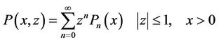
1) New customers arrive in batches according to a compound Poisson process with rate λ. Let Xk denote the number of customers belonging to the kth arrival batch, where Xk, k = 1, 2, 3, ∙∙∙ are with a common distribution

and X(z) denotes the probability generating function of X.
2) The server provides one phases service to each customer. The service discipline is assumed to be first come first served (FCFS). Further, the service time is random variable B, with distribution function , Laplace transform
  and finite moments
  for l ≥ 1 .
3) After completion of any customer’s service, the server may take a vacation with probability θ or may continue to be in the system with probability 1 – θ.
We assume that the vacation time has two phases with phase one is compulsory. However, after phase 1 vacation, the server takes phase 2 vacation with probability p or may return back to the system with probability 1 – p. The vacation times are random variables Vi for i = 1, 2, follows a general law of probability with distribution function , Laplase transform
  and finite moments
  for k ≥ 1.
4) There is an admissibility restricted policy for batches in which not all batches are allowed to join the system at all times. Let α (0 ≤ α ≤ 1) and β (0 ≤ β ≤ 1) be the probability that an arriving batches will allowed to join the sysytem during the period of server’s busy and vacation times respectively.
5) The random variables B, V1 and V2 are independent.
Definition 2.1 The modified service time or the time required by a customer to complete the service cycle is given by
 (1)
(1)
where
 (2)
(2)
then the LST  of
of  is given by
 (3)
(3)
and
 (4)
(4)
also
 (5)
(5)
where
 (6)
(6)
also
 (7)
(7)
Further we assume ,
,  and
and  is continuous at
 , so that
 (8)
(8)
is the hazard rate function of B.
Also for i = 1, 2 we assume ,
,  and
and  are continuous at
 . The hazard rate functions of
 ’s are
 (9)
(9)
Definition 2.2 The elapsed time of service at time “t” is denoted by . For i = 1, 2, also
  denote the elapsed time of vacation time at time “t”, and
  denote the queue size at time “t”. For i = 1, 2 we introduce the random variable
  as follow:
 (10)
(10)
Then we have a bivariate Markov process  where
where  if
if ;
;  if
if ;
;  if
if  and
and  if
if .
.
Now for i = 1, 2 the following probabilities defined as
 (11)
(11)
 (12)
(12)
and
 (13)
(13)
With assumption that steady state exist, we let
 (14)
(14)
 (15)
(15)
 (16)
(16)
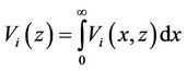
Now for i = 1, 2 the PGF of this probabilities are defined as follow:
 (17)
(17)
 (18)
(18)
Also
 (19)
(19)
 (20)
(20)
3. Steady-State Probability Generating Function
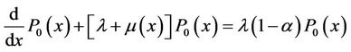
From kolmogorov forward equations, for i = 1, 2 the steady-state conditions can be written as follow
 (21)
(21)
 (22)
(22)
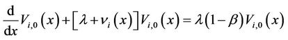
 (23)
(23)
and
 (24)
(24)
also
 (25)
(25)
At  for
for  the boundary conditions are
 (26)
(26)
 (27)
(27)
also
 (28)
(28)
Finally the normalizing condition is
 (29)
(29)
Lemma 3.1 The solution of first order Equation (21) is
 (30)
(30)
and for i = 1, 2 the solution of first order Equation (23) is
 (31)
(31)
Proposition 3.2 If for i = 1, 2
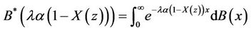 (32)
(32)
 (33)
(33)
are the z-transforms of B and  respectively, then
 (34)
(34)
 (35)
(35)
 (36)
(36)
 (37)
(37)
 (38)
(38)
Proof:
1) Since

then by integeration from (30) by part the result obtained.
2) Since for i = 1, 2
then from (31) similarly we have 2).
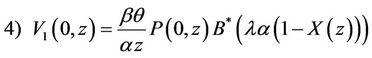
3) First multiply (26) in  and summation from n = 1 to
 , then using (25) we obtain result.
4) By multiplying (27) in  and summation from n = 0 to
  the result obtained .
5) By using the same technique on (28), we have 5).
In the rest of this section for simplifying we omit  from
from  and
and  from
from
 .
.
Corollary 3.3
1) By using (37), (38) in (36) we have
 (39)
(39)
2) By using (39) in (37) we have
 (40)
(40)
3) By using (41) in (38) we have
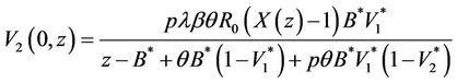 (41)
(41)
Corollary 3.4 1) By substituting (39) in (34) we have
 (42)
(42)
and for i = 1, 2 substituting (40) and (41) in (35) result
 (43)
(43)
 (44)
(44)
For calculating , by using the normalizing condition (29) we have
 (45)
(45)
 is the steady-state probability that the server is idle but available in the system , hence if
  be the stability condition under which the steady state solution exist, then
  and by using (42), (43), (44) with L’Hopital we have

and
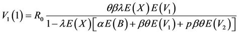

By substituting this values in (45) we have , where
 (46)
(46)
Now the PGF of the queue size at a random epoch is
 (47)
(47)
The PGF of the system size is
 (48)
(48)
Remark 3.5 In this system we set

then

This is familiar with famous formula Pollaczek-Khinchin in M/G/1 queue for PGF of system’s queue size.
4. Mean Queue Size
Let L be the mean number of customers in the system, then we have
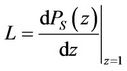 (49)
(49)
Proposition 4.1 From (49) and using (48) we have
 (50)
(50)
where  and
and  are in (6) and (7).
Proof:  has the form
 , where

and
Since , then by using L’Hopital’s rule, we have
 (51)
(51)
where  and
and  is in (46).
Also


and by using (6) and (7)

hence by substitute this value in (51) the result obtain.
5. Mean Response Time
The response time  is the time interval from the arrival time of a test customer to the time when it leaves the system after service completion i.e., waiting time plus service time.
By using Little’s formula, this measure of system is

where following the admissibility assumption of our model,  the actual arrival rate of batches is given by
 (proportion of non-vacation time) +
 (proportion of vacation time).
But the proportion of vacation time is

and hence the proportion of non-vacation time is  . Consequently
 (52)
(52)
6. Special Cases and Numerical Results
Analyzing a queueing system via actual cases are very important and an useful way for confirm the models. In this section we chose known distributions for service time and vacation times, so with this and by sum numerical approches the validity of system examained. Also this approch explain that our model can represent some practical problems reasonably well.
Case 1: Let the distribution of service time is  -Erlang as follow

hence

so  and
and . Also we assume the distribution of vacation times respectively are

hence

so  and
and . If we chose geometric distribution for batch size, i.e.
 ,
,  , then
 .
.
Now for numerical result we assume the following values for parametrs such that the steady state condition ( ) obtained.
In this case using above values and (46), if  then
then  with respect
  and hence steady state condition is
 , so
, so . By using (50)

Table 1 shows some values of L with respect θ, in which L increases with respect θ with a mild gradient.
Also Figure 1 show the mild curve of L with respect θ.
Now we analyze L against . Using the values of Table 2, if
  then steady state condition is
  or
or .
.
Also L with respect  is
is

Figure 2 shows L agains . Near
  the system blowing up. Untile 2 customers the system is stable.
Case 2: In this case we assume the distribution of service time and for i = 1, 2 vacation times are exponential as follow


With geometric distribution for batch size and following values for parameters in Table 4 the steady state condition is  or
or . Also

and the graph of model is in Figure 3. According to this curve, L decresses with respet , and after
  the system is stable.

Figure 1. L vis-a-vis θ.

Figure 2. L vis-a-vis λ.

Table 1. Values of L with respect θ.

Table 2. Values of parameters.

Table 3. Values of L with respect λ.

Table 4. Values of parameters.

Table 5. Values of L with respect μ.

Table 6. Values of parameters.

Table 7. Values of L with respect θ.

Figure 3. L vis-a-vis μ.
Also Table 5 shows some values of L against μ. When μ incresses from 1.5 to 2, then system changed in stable form.
In this case we assume θ is unknown. With the values in Table 6 the steady state condition is  or
or .
.
Also

Table 7 shows some values of L against θ. After , the system blowing up.
Case 3: In this case we assume the service time has deterministic distribution. Hence it is sufficient 
in case 1, and distribution degenerates in . Also if
 and
and  then steady state is

or
 .
.
In this case we obtain the results of [9].
7. Concluding Remarks
In this paper we have studied a batch arrival queueing sysytem with admissibility restricted and optional server’s vacation which generalized classical M/G/1 queue. An application of this model can be found in mobile network where the messages are in batch form, the system may have two phases vacation such that first phase is essential but the second phase may chosen randomly and have optional cases. Also because of admissibility restriction in service or system all batches don't enter in service. Our investigations concered with not only queue size distribution but also waiting time ditribution. Also by some numerical approches the validity of results are examined. A practical generalization for this system is to consider optional service.
REFERENCES
- J. Keilson and L. D. Servi, “Dynamic of the M/G/1 Vacation Model,” Operations Research, Vol. 35, No. 4, 1987, pp. 575-582.
- Y. Baba, “On the Mx/G/1 Queue with Vacation Time,” Operations Research Letters, Vol. 5, No. 2, 1986, pp. 93- 98. doi:10.1016/0167-6377(86)90110-0
- K. C. Madan and W. Abu-Dayyeh, “Restricted Admissibility of Batches into an Mx/G/1 Type Bulk Queue with Modified Bernoulli Schedule Server Vacations,” ESSAIMP: Probability and Statistics, Vol. 6, No. 2, 2002, pp 113- 125. doi:10.105/ps:2002006
- K. C. Madan and W. Abu-Dayyeh, “Steady State Analysis of a Single Server Bulk Queue with General Vacation Time and Restricted Admissibility of Arriving Batches,” Revista Investigation Operational, Vol. 24, No. 2, 2003, pp. 113-123.
- K. Alnowibet and L. Tadj, “A Quarum Queueing System with Bernoulli Vacation Schedule and Restricted Admissibility,” Advanced Modeling and Optimization, Vol. 9, No.1, 2007, pp.171-180.
- K. C. Madan and G. Choudhury, “An Mx/G/1 Queue with a Bernoulli Vacation Schedule under Restricted Admissibility Policy,” Sankhya, Vol. 66, No. 1, 2004, pp 175-193.
- G. Choudhury, “A Note on the Mx/G/1 Queue with a Random Set-Up Time under a Restricted Admissibility Policy with a Bernoulli Vacation Schedule,” Statistical Methodology, Vol. 5, No. 1, 2008, pp 21-29. doi:10.1016/j.stamet.2007.03.002
- A. Badamchi Zadeh, “An Mx/(G1, G2)/1/G(BS)Vs with Optional Second Services and Admissibility Restricted,” International journal of Information and Management Sciences, Vol. 20, No. 2009, pp. 305-316.
- K. C. Madan and A.-J. Jehad, “Steady State Analysis of an M/D/1 Queue with Coxian-2 Server Vacations and a Single Vacation Policy,” Information and Management Sciences, Vol. 13, No. 4, 2002, pp 69-81.
- B. T. Doshi, “Queueing System with Vacation—A Survey,” Queueing Systems, Vol. 1, No. 1, 1986, pp 29-66. doi:10.1007/BF01149327
- D. Gross, J. F. Shortle, J. M. Thompson and C. M. Harris, “Queueing Theory,” Wiley, Hoboken, 2008.