Journal of Applied Mathematics and Physics
Vol.06 No.09(2018), Article ID:87356,23 pages
10.4236/jamp.2018.69158
SPH Particle Collisions for the Reduction of Particle Clustering, Interface Stabilisation and Wall Modelling
Arno Kruisbrink1, Stan Korzilius2*, Frazer Pearce1, Hervé Morvan1
1Gas Turbine and Transmission Research Centre, University of Nottingham, Nottingham, UK
2Centre for Analysis, Scientific Computing and Applications, Eindhoven University of Technology, Eindhoven, The Netherlands

Copyright © 2018 by authors and Scientific Research Publishing Inc.
This work is licensed under the Creative Commons Attribution International License (CC BY 4.0).
http://creativecommons.org/licenses/by/4.0/


Received: July 9, 2018; Accepted: September 15, 2018; Published: September 18, 2018
ABSTRACT
The pair-wise forces in the SPH momentum equation guarantee the conservation of momentum, but they cannot prevent particle clustering and wall penetration. Particle clustering may occur for several reasons. A fundamental issue is the tensile instability, which is caused by negative numerical pressures. Clustering may also occur due to certain properties of the kernel gradient. Discontinuities in the pressure and its gradient, due to surface tension and gravity, may cause particle instabilities near the interface between two fluids. Wall penetration is also a form of particle clustering. In this paper the particle collision concept is introduced to suppress particle clustering. Here, the use of kinematic conditions (motion) rather than dynamic conditions (forces) is explored. These kinematic conditions are obtained from kinetic collision theory. Conservation of momentum is maintained, and under elastic conditions conservation of energy as well. The particle collision model only becomes active when needed. It may be seen as a particle shifting method, in the sense that the velocities are changed, and as a consequence of that the particle positions change. It is demonstrated in several case studies that the particle collision model allows for realistic (low) viscosities. It was also found to stabilise the interface between two fluids up to high, realistic density ratios (1000:1) in typical liquid-gas applications. As such it can be used as a multi-fluid model. The concept allows for real wave speed ratios (and far beyond), which, as well as real viscosities, are essential in the modelling of heat transfer applications. The collisions with walls allow for no-slip conditions at real viscosities while wall penetration is suppressed. In summary, the particle collision model makes SPH more robust for engineering.
Keywords:
SPH, Particle Clustering, Multiphase Flow, Interface Stabilisation, Wall Modelling

1. Introduction
Smoothed particle hydrodynamics (SPH) is a numerical, Lagrangian method to simulate fluid flows. It was invented by Gingold and Monaghan [1]and Lucy [2]to simulate astrophysical problems, but it is gaining popularity in engineering as well [3]. The key concept of SPH is that a function value at a specific point in the domain is estimated from surrounding points by means of a smoothing kernel. To that end, interpolation points are introduced that―owing to the Lagrangian nature of the method―move with the flow. The interpolation points also carry mass and other properties and are therefore called particles.
The clustering of particles remains an issue in SPH that affects the stability, which is one of the grand challenges defined by the SPHERIC Steering Committee. Particle clustering reduces the resolution of the simulation, which―besides making it a waste of computational effort [4]―endangers the accuracy of the results. It is thus of great importance to reduce the numerical clustering of particles as much as possible. There is somewhat confusion about the cause of this phenomenon. This is due to the presence of two types of particle clustering. On the one hand there is the tensile instability [5][6]; this instability can occur in simulations that allow for negative pressures. On the other hand, there is the pairing or clumping instability, which is caused by a vanishing repelling force for approaching particles.
The vanishing repelling force is the result of the flat shape of most commonly used kernels for inter-particle distances close to zero. This implies that for very small distances the kernel gradient tends to zero and as a consequence the (repulsive) pressure force vanishes. This makes that particles that happen to be close will stay close, unless some other force separates them. That is one of the reasons that artificial viscosity was introduced [7][8]. Later on, algorithms were developed to introduce artificial viscosity around shocks only [9][10][11], this way reducing the amount of artificial viscosity in other areas of the flow. Monaghan also introduced an inter-particle repulsive force similar to the Lennard-Jones force [5]. Remeshing as described by Chaniotis et al. [12]also prevents particles from clustering, but it has disadvantages as well. It implies interpolation, which affects the accuracy and makes it computationally expensive. Moreover, with remeshing SPH loses one of its biggest advantages: not having a predefined mesh. Another remedy for the vanishing repelling force is a convex kernel function that does not have a flat central portion. Such kernels have been introduced by, e.g. Schussler and Schmitt [13]; Johnson and Beissel [14]; Read et al. [15]; Korzilius et al. [16]and were reported to reduce the clustering of particles. Despite this property, convex kernels are rarely used in literature. This is mainly because, due to their different weight distribution, convex kernels perform worse in the density estimate [4][16][17].
Particle clustering may also occur at the interface between two fluids, due to changes in pressure (e.g. due to surface tension) and pressure gradient (due to gravity), the latter in particular at high density ratios. To deal with the particle instability at an interface, multi-fluid models are introduced by, e.g. Colagrossi et al. [18], Monaghan [19]and Kruisbrink et al. [20]. In the number density approach [18]the wave speed of the high density fluid must be chosen lower than that of the low density fluid to make the algorithm stable. The multi-fluid model of Monaghan [19]is based on a repulsive force between particles of different fluids. At high density ratios the wave speed of the low-density fluid is still a factor 5 to 7 higher than that of the high-density fluid. With the quasi-buoyancy model of Kruisbrink et al. [20][21], much more realistic wave speed ratios (close to reality) can be applied in gravity dominated problems. Although the wave speeds may be artificial in many cases, correct and realistic wave speed ratios are essential in the modelling of heat transfer between two fluids.
Particle clustering is also seen in incompressible SPH (ISPH). Particles move along streamlines when the pressure is solved accurately, which leads to stretching and compressing [22], so that particle clustering (e.g. near stagnation points) cannot be avoided [23]. As a remedy, Xu et al. [22]introduced a particle shifting method, based on the anisotropy of the particle spacing, while the shifting magnitude is based on coefficients. This approach is followed by Lind et al. [23][24], who based the shifting however on Fick’s law of diffusion. Particles are shifted from regions of high concentration to regions of low concentration, based on a diffusion or shifting coefficient. In the concentration gradient a tensile instability term is included, also based on coefficients. In their combined incompressible-compressible SPH approach, the particle shifting is applied to the incompressible phase, while artificial viscosity is used to stabilise the compressible phase. As such the particle shifting method is not a multi-fluid model for interface stabilisation, nor is it used to allow for real (low) viscosities. Furthermore, the shifting algorithm violates the conservation of momentum in SPH [24].
Except for the remeshing and shifting algorithms, all above mentioned methods are based on forces. Unfortunately, this cannot guarantee that particle clustering does not occur. In this paper we propose a kinematic concept based on particle collisions. The idea of collisions in SPH is not entirely new [25][26], but to our knowledge has not been applied in the way we propose. The model is derived from kinetic collision theory, satisfying conservation of momentum (for inelastic and elastic collisions) and energy (for elastic collisions). The concept takes the form of a typical SPH viscosity model. It directly influences the approach velocities of particles and is therefore more robust than dynamic concepts based on forces.
The paper is arranged as follows. In Section 2 the basic equations of our particle collision model are derived from kinetic collision theory. Both inter-particle collisions and particle collisions with walls are considered. In Section 3 the equations are applied within the SPH concept. Further the criteria are described under which the particle collisions are applied. Also, an analogy between our collision model and existing SPH viscosity models is shown. In Section 4 an overview is given of the SPH models as used in the case studies. Our collision model is then applied and tested in Section 5, in four cases with their specific characteristics. The first case, the Taylor-Green vortex, is a well-known case to study the decay of energy due to viscosity. The second case focuses on the interface stabilisation of the stagnant flow in a reservoir with two fluids at high density ratios. The third case is a dam break, a classical SPH benchmark with high dynamics, here simulated as a multi-fluid flow. In the last case the focus is on wall boundary treatments in the simulation of a jet impinging on a wall. Finally, in Section 6, a summary is given together with the main conclusions of our findings.
2. Kinetic Collision Theory
In this section the kinetic collision theory is described, which is applied to SPH in Section 3. Consider two colliding particles i and j. Denote the approach velocities of the particles by , while , are the separation velocities after the collision.
2.1. Inter-Particle Collision
Within kinetic collision theory a distinction is made between elastic and inelastic collisions. During an elastic collision no energy is dissipated, so that both the conservation of momentum and the conservation of energy are satisfied. This may be formulated as:
(1)
and
(2)
Solving for gives:
(3)
and a similar expression for .
During an inelastic collision energy is dissipated, while in the limit case of a fully inelastic collision the separation velocities are equal. This may be formulated as:
(4)
with the velocity of particles i and j. Thus, for the velocity of particle i after the collision we have:
(5)
with the same expression for .
Combining the results for an elastic and inelastic collision in Equations (3) and (5) yields:
(6)
where is the coefficient of restitution, representing the elasticity of the collision. For an inelastic collision and for an elastic collision . For the change of velocity of particle i due to the collision it follows after some manipulation that:
(7)
where “®” should be read as “due to collision with”. This directly shows that the total change of momentum is zero, i.e. . The above derivation can be extended to more than two particles. For an arbitrary number of collisions, (7) becomes:
(8)
where is the sum of masses of the particles with which particle i collides. The collision of more than two particles within a time step is rare, provided that the time step is chosen sufficiently small. However, if it occurs, it must be dealt with. The modelling of serial collisions is possible but computationally expensive, while the serial treatment does not fit within the pairwise treatment in SPH. Therefore the (rare) multiple collisions are assumed to take place simultaneously.
2.2. Particle Collision with Wall
The collision of a particle with a wall is very similar to that with another particle. The mass of the wall may be considered to be infinite and the wall velocity is zero, or non-zero for a moving wall. In that case Equation (8) reduces to ( ):
(9)
(10)
where is the coefficient of restitution for collisions with a wall, which may differ from the coefficient of restitution for inter-particle collisions, .
3. Application to SPH
3.1. Inter-Particle Collision
The collision theory in the previous section is applied in the inter-particle direction only; the velocity components in the other directions remain unchanged. The relative approach velocity of particles i and j is given by:
(11)
where is the relative velocity vector of particle i and j, is the relative position vector, is the distance between the particles and is the unit vector in the direction of , i.e. . Substituting Equation (11) into Equation (8) leads to:
(12)
Simulations have shown that in most cases a particle will collide with only one particle, provided that the time step is sufficiently small. For a single collision (12) reduces to:
(13)
where denotes the velocity change of particle i due to a collision with particle j. Equation (12) is introduced as the particle collision model, which is easy to implement within the SPH framework. It describes the total change of velocity of particle i due to collisions with its direct neighbours. Note that the duration of the collision is not described. The contact time may be very short, all we know is that it takes place within one time step.
3.2. Particle Collision with a Wall
The collision of fluid particles with walls is very similar to that with other particles. Walls can be modelled by ghost particles, wall particles or a continuous wall. Each concept needs a slightly different treatment.
Collisions with ghost particles are similar to those with fluid particles, except that the (virtual) mass of ghost particles is assumed to be infinite, so that their velocity remains unchanged (i.e. zero or non-zero for a moving wall). It is assumed that the distance between ghost particles is such that a fluid particle can collide with only one ghost particle at the same time. In that case Equation (13) reduces to:
(14)
For collisions with wall particles the approach velocity is no longer evaluated in the inter-particle direction but in the direction normal to the wall, while the mass is again assumed to be infinite. In that case we obtain:
(15)
where is the unit vector normal to the wall. The same formulation holds for collisions with a continuous wall (virtual wall without particles). Note that the virtual mass is only applied within the particle collision concept, since ghost particles must have the same properties as fluid particles to allow for a proper density estimate.
Particle collisions may help to ensure that wall boundary conditions are satisfied. To allow for a no-slip condition the velocity component parallel to the wall should equal the wall velocity. This is achieved in a fully inelastic collision ( ) when ghost particle are used to represent the wall. To allow for a free-slip condition the velocity component parallel to the wall should not be affected. This is achieved in the case of wall particles or a continuous wall for any value of .
3.3. Criteria for Particle Collision
The particle collision concept should not affect the pressure and should only be applied outside the range of (minimum and maximum) real pressures. It is therefore only applied at high pressures, equivalent with small particle distances, and under compression. These conditions are described by:
(16)
where is the collision distance at which particle collisions become active. It may be defined as , where is the natural particle distance under zero (reference) pressure conditions and is the collision distance parameter. To evaluate the collision distance, the pressures are related to particle distances via:
(17)
where V is the particle volume, c is the (artificial) wave speed, while the subscript 0 refers to reference values. The collision distance must be chosen smaller than the minimum particle distance occurring at maximum pressure. This leads to:
(18)
The collision distance depends on the (artificial) wave speed, and can be evaluated from an estimate of the real maximum pressure in each case.
Furthermore, to allow for a shear flow, the collision distance should be smaller than the particle distance in the direction perpendicular to the flow. For a hexahedral particle distribution this means that .
3.4. Analogy with SPH Viscosity Models
To show the analogy with force-based concepts, we introduce the contact time during a collision, . It now follows from Equation (12) that:
(19)
This formulation allows for a comparison with viscous forces. The form of a typical SPH viscosity model is:
(20)
where the viscosity term can be described in several ways. In the Monaghan artificial viscosity model the linear term is [7][27]:
(21)
where , and . In the Monaghan real viscosity model this term is [27][28]:
(22)
Here, and (the factor 1/8 being valid in two dimensions).
A comparison of Equations (19) and (20) learns that the formulation of the force due to a collision shows an analogy with a viscous force, although it does not depend on a smoothing kernel. In that sense the concept may be considered as a time dependent SPH viscosity model. However, the essential difference is that the repulsive force may become extremely high, since the collision may take place in a very short period, within a fraction of the SPH time step. The duration of the collision is not known (at least not within SPH), but its effect (i.e. the change of velocities) is easily described.
4. SPH Model Equations
In SPH, function values at particle positions are approximated by weighted sums over the function values of the surrounding particles:
(23)
Here, is the volume of particle j, which is usually substituted by , where represents the density. The sum is taken over all particles j, with masses , and is a smoothing kernel whose value depends on the distance between particles and the smoothing length h. Examples of smoothing kernels are the Gaussian kernel―originally used by Gingold and Monaghan [1]; Monaghan [29]―and the widely used cubic spline [27]. In this paper we use a kernel function derived by Wendland [30]:
(24)
for and zero otherwise. In two dimensions, the normalisation factor equals . Spline functions and Wendland kernels have the advantage of compact support, reducing the computational expense.
In weakly compressible SPH an incompressible fluid is considered to be slightly compressible. When the gradient of Equation (23) is applied to the velocity, the resulting estimate can be substituted in the continuity equation. This gives an approximation for the density in the form of an evolution equation:
(25)
This SPH version of the continuity equation leads to better results than the summation density in case of free surface flows and (high density ratio) multiphase flows. When the densities are known, the pressures are obtained from the equation of state:
(26)
where is the polytropic exponent. Equation (26) is often misquoted as the Tait equation, since it was already proposed in a similar form by Murnaghan [31], as also noted by Gilvarry [32]and MacDonald [33]. When the pressures are known, the pressure gradients are obtained from the discrete momentum equation. Various forms are available. In this paper we use:
(27)
Here, is a viscosity term for which we use the formulation in Equation (22). Equations (25) and (27) form a consistent set of equations according to the variational principle [4]. For more details on the theory and equations of SPH we refer to [4][29][34].
5. Case Studies
In this section the particle collision concept is explored in four case studies. In all cases we model either water ( kg/m2), air ( kg/m2), or both. The following five cases are considered: The Taylor-Green vortex, a well-known case in the literature; the hydrostatic case of a reservoir with air on top of water, which allows us to focus on the interface between fluids at a high density ratio; the multi-fluid dam break problem, a classical SPH benchmark case; the jet impinging on a wall, in which wall collision concepts are explored.
For convenience and readability we state here the parameters that have the same values in the case studies, unless mentioned otherwise. For both air and water we use the real viscosity term given in Equation (22), with values and . In the equation of state we use and . We use the kernel function in Equation (24), with a constant smoothing length of . For time integration we use the Explicit Euler method, which is stable if the time steps are sufficiently small. It is only first order accurate, but it allows for a comparison with standard SPH (i.e. the model equations in Section 4) and that with the particle collision concept (described in Section 3). The velocity change due to a collision in Equation (12), is applied together with the integration of the particle acceleration in Equation (27). In all simulations the initial particle distribution is hexahedral, which is the natural (most dense) distribution under stagnant flow conditions.
5.1. Taylor-Green Vortex
The Taylor-Green vortex is an unsteady flow of a decaying vortex, which has an exact solution of the incompressible Navier-Stokes equations. The benchmark case is used for testing and validation of SPH algorithms by e.g. Hu and Adams [35][36]. In the two-dimensional case the velocity field may be described by:
(28)
where is the velocity amplitude and L is the domain size, while the decay is represented by the exponent . The Reynolds number is defined as . The pressure field can be obtained by substituting the solution for the velocity field in the momentum equation. This yields:
(29)
We use air particles with m/s, and in the equation of state (26). The domain size is m and the velocity amplitude m/s―so that ―which are the same values as used by Hu and Adams [36]. The above solution for the velocity and pressure field at is used as initial condition in the SPH simulations. Figure 1 shows the initial condition on a grid, so that the initial velocity field is clearly visible.
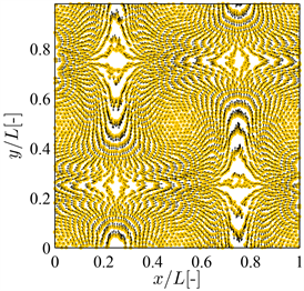
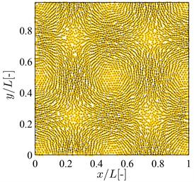
The actual SPH simulations are performed on an (initial) hexahedral grid of particles. The simulation with standard SPH, shown in Figure 2(a), shows large areas of particle clustering and layering, which are strongly reduced in the simulation with particle collisions (Figure 2(b)).
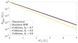
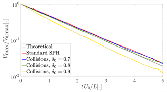
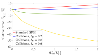
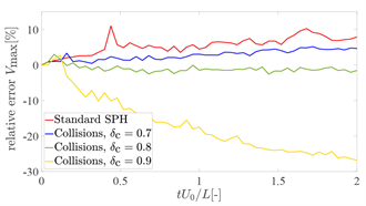
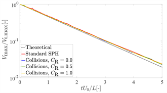
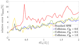
For the Taylor-Green vortex analytical solution exist for the decay of kinetic energy and maximum fluid velocity in time. In Figure 3 the effect of the collision distance, represented by the collisions distance factor , on the decay is shown versus the dimensionless time, while the restitution coefficient is kept constant at . In all cases the decay of kinetic energy agrees reasonably well with theory, except for . Note that in this case , so that the criteria for particle collisions (see Section 3.3) are not satisfied. With standard SPH, the maximum velocity exceeds the theoretical one. In the beginning of the simulation this is revealed by the peak value in the relative error (Figure 3(d)), which may fully be attributed to the particle clustering and
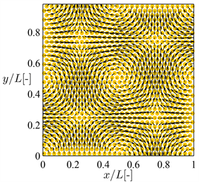
Figure 1. Taylor-Green vortex. Initial condition, shown here on a grid, so that the velocity field is clearly visible.
 (a)
(a)
 (b)
(b)
Figure 2. Taylor-Green vortex ( ). Simulations are shown at without and with particle collision concept. In the latter case, and . (a) Standard SPH; (b) With particle collisions.
layering seen immediately after the start of the simulation (Figure 2(a)). With particle collisions the relative errors are reduced as long as , while they are the smallest for (less than about 2%).
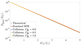
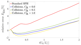
In Figure 4 the effect of the restitution coefficient on the decay of kinetic energy and maximum velocity is shown, while the collision distance factor is kept constant at . Here, in all cases the decay of kinetic energy agrees well with theory, while the maximum velocity is slightly overestimated. Also here standard SPH shows a peak value in the relative error (Figure 4(d)), which does not appear with particle collisions. The relative errors are significantly reduced for all CR-values. The relative error in the maximal velocity (up to 4%) is slightly higher than that in the results of Hu and Adams [35](up to 3%) at the same resolution. The latter results are obtained with ISPH, where a reference or background pressure is used, which is superimposed on the pressure to avoid stability problems due to negative pressures.
 (a)
(a)
 (b)
(b)
 (c)
(c)
 (d)
(d)
Figure 3. Taylor-Green vortex ( ). Effect of the collision distance (at constant ) and a comparison of standard SPH and particle collisions on the decay of total kinetic energy and maximum velocity. and are the energy and maximum velocity at . (a) Kinetic energy; (b) Maximal velocity; (c) Relative error kinetic energy; (d) Relative error maximal velocity.
 (a)
(a)
 (b)
(b)
 (c)
(c)
 (d)
(d)
Figure 4. Taylor-Green vortex ( ). Effect of the restitution coefficient (at constant ) and a comparison of standard SPH and particle collisions on the decay of total kinetic energy and maximum velocity. and are the energy and maximum velocity at . (a) Kinetic energy; (b) Maximal velocity; (c) Relative error kinetic energy; (d) Relative error maximal velocity.
Summarising, the particle collision concept suppresses particle clustering and layering. It reduces the relative errors in the decay of total kinetic energy and maximum velocity, as long as the collision distance satisfies the criterion (see Section 3.3).
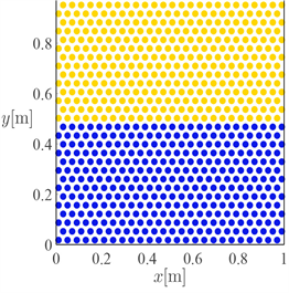
5.2. Stagnant Flow in a Reservoir
The second case is a stagnant, multi-fluid flow under gravity. The lower half of a reservoir is filled with water, while the upper half consists of air. The bottom wall of the reservoir is represented by ghost particles which, apart from their fixed positions, act like fluid particles. The two vertical walls of the reservoir are modelled by periodic boundaries. The initial particle spacing is , which gives a total of approximately 800 particles. In our simulations we use a realistic wave speed ratio of 4, whereby it should be noted that the wave speed of water is chosen higher than that of air ( ). Although this is physically correct, it is usually not done in SPH. In the number density approach [37]the wave speed ratio at a density ratio of 1000:1 is chosen as 1:14, so that the compressibility of the two fluids is the same. This is necessary to stabilise the algorithm. This is improved in the multi-fluid algorithm of Monaghan [19], but the wave speed of air is still a factor 5 to 7 higher than that of water.
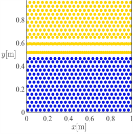
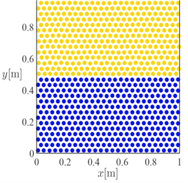
Some typical results are shown in Figure 5. Simulations are performed without and with the particle collision concept, in the latter case with and .
Without treatment the interface becomes unstable soon after the start of a simulation, which is revealed by the clustering of particles (Figure 5(b)). With particle collisions the interface remains stable for a time scale that is at least one order of magnitude larger (Figure 5(c)). From other simulations it is concluded that the interface becomes slightly more unstable with increasing wave speed ratio, as may be expected. However, it still remains intact, even at an (unrealistic) high wave speed ratio of 20. Note that in reality, like in our simulations, the wave speed ratio of water and air is about 4 ( m/s and m/s at 20˚C).
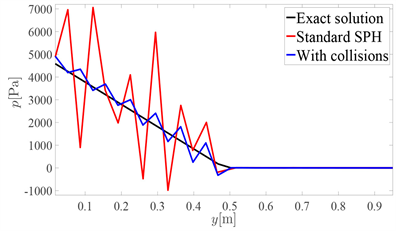
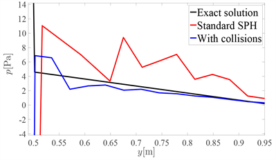
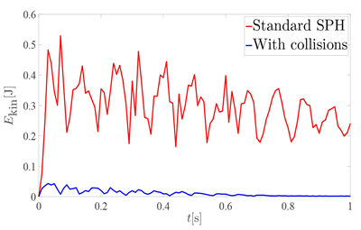
Figure 6 shows the pressure distribution for the simulations in Figure 5. Without interface treatment, the pressure is fluctuating heavily around the physically correct pressure. With the collision concept, the pressures are much closer to the (initial) linear pressure distribution. In Figure 7 the results of a stability analysis are shown, where the evolution of total potential and kinetic energy of the water-air system is plotted in time. With standard SPH the potential energy immediately drops after the start of the simulation. Potential energy is converted into kinetic energy, indicating that the particles are moving and they keep moving. With particle collisions the initial drop of potential energy is much smaller and coupled with a slight increase of kinetic energy. This results in a slight move of the particles until the collisions prevent any further movement. The total kinetic energy then returns to zero.
 (a)
(a)
 (b)
(b)
 (c)
(c)
Figure 5. Stagnant flow in a reservoir. Gravity acts vertically downwards, with the lower half water and the upper half air. The wave speed ratio between the two fluids is 60:15. Static ghost particles are placed below the tank, while the top is left open. A comparison of standard SPH and particle collisions ( ). (a) Initial condition; (b) Standard SPH (t = 0.05 s); (c) With collisions (t = 1.0 s).
 (a)
(a)
 (b)
(b)
Figure 6. Stagnant flow in a reservoir. Average pressures as a function of particle height. Comparison of standard SPH and the particle collision model. (a) Full reservoir; (b) Top part of reservoir.
 (a)
(a) 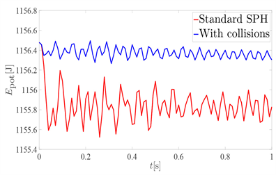 (b)
(b)
Figure 7. Stagnant flow in a reservoir. Stability analysis with the evolution of total potential and kinetic energy of the water-air system in time. Comparison of standard SPH and the particle collision model. (a) Potential energy; (b) Kinetic energy.
5.3. Multi-Fluid Dam Break
The two-dimensional dam break is a classical SPH benchmark case (e.g. [3][37][38][39][40]), which is usually simulated as a single phase flow. Here, we consider a multi-fluid dam break with a density ratio of 1000:1. The setup is as in [37][41], but with air particles surrounding the water. The domain boundary consists of ghost particles which have a constant density equal to the initial density of the water particles. The initial particle spacing is chosen such that we have approximately the same number of water particles as Antuono et al. [41]. In total we have over 38,200 particles. The wave speeds for water and air are 60 and 15 m/s, respectively.
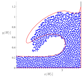
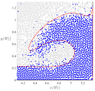
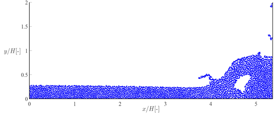
Figure 8 shows the flow at . The water particles are depicted in blue, the air particles in grey. The red lines, shown in all panels, give the BEM solution given in [41]. Figure 8(a) shows the single-fluid simulation of Antuono et al. [41]without extra diffusive terms, to allow for a more honest comparison with our results. The simulation with standard SPH (Figure 8(b)) captures the free surface contour reasonably well. Note that we did not use any remedies, like diffusive terms, density re-initialisation, artificial viscosity terms, XSPH correction, control of interface sharpness or adapted state equations, as used by other researchers (e.g., Colagrossi and Landrini [37]), neither did we use a high-order time stepping scheme. Therefore the particle distribution itself is also very noisy. However, with collisions ( and , Figure 8(c)) the shape of the wave is captured quite well. Increasing the restitution to increases the dynamics, which has a negative effect on the particle distribution and leads to results similar to those without collisions. A larger collision distance keeps particles closer together, but also makes the flow a bit more viscous (Figure 8(d)).
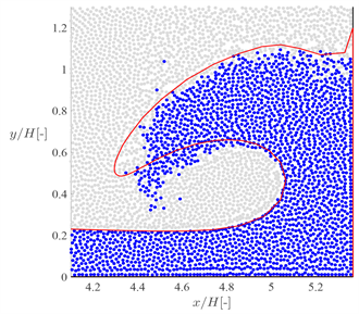
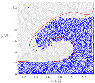
At , the breaking wave has plunged back into the flowing water, as shown in Figure 9. Figure 9(a) again shows the single-fluid results of Antuono et al. [41]without diffusive terms. Our multi-fluid simulations with particle collisions are very similar and capture the shape of the wave very well. Note again that we did not need to use the above mentioned remedies to be able to simulate this multi-fluid flow, simply including the collision concept was sufficient. A small white area in the bottom panel just below the water stream that has bounced back up indicates a small cavity. This cavity does not appear when .
5.4. Jet Impinging on Wall
The jet impinging on a wall is a steady flow case, which is characterized by a diversion resulting in two flows moving in opposite directions along the wall. An exact analytical solution exists for inviscid fluids with a free slip wall condition. The case is used for validation of SPH models by other researchers, e.g. Antuono et al. [42]. Here it is used to demonstrate that the particle collision model can be applied to impose free-slip as well as no-slip wall boundary conditions.
For an inviscid and incompressible fluid the diversion of the jet along the wall can be derived from the momentum (Bernoulli) and continuity equations,
 (a)
(a)
 (b)
(b)
 (c)
(c)
 (d)
(d)
Figure 8. Dam break flow at . The top left panel shows the single-fluid results of Antuono et al. [41]when no diffusive terms are used, while the top right panel shows the standard multi-fluid SPH solution. The bottom panels show the multi-fluid results with particle collisions for different choices of the collision parameters. The red lines show the BEM solution of Antuono et al. [41]. (a) Solution of Antuono et al. [41]; (b) Standard SPH; (c) With collisions ( ); (d) With collisions ( ).
neglecting energy losses in the impact and wall regions. The free surface contours are given by [43]:
(30)
(31)
 (a)
(a)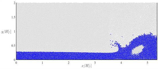 (b)
(b)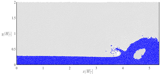 (c)
(c)
Figure 9. Dam break flow at . The top panel shows the single fluid results of Antuono et al. [41]without diffusive terms. The other panels show multi-fluid results of the particle collision concept for different choices for the collision parameters. (a) Solution of Antuono et al. [41]; (b) With collisions ( ); (c) With collisions ( ).
where is the width of the jet, is the inclination angle and:
(32)
The second term in the y-coordinate of the free surface contour vanishes far from the impingement ( , ), where the height of the left and right branches is constant, as described by the first term. Here the magnitude of the flow velocity is the same as the jet velocity.
In all simulations the width of the water jet is m, the inclination angle defined from the wall is , the real viscosity Ns/m2. The wave speed is chosen ten times higher than the jet velocity. The initial particle distance is chosen such that . The wall is represented by ghost particles.
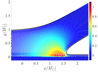
First, we demonstrate that the collision wall allows for a free-slip wall condition, while it also suppresses wall penetration. In this case the viscosity of the ghost particles is set to zero. To suppress the noise in the pressure distribution, Antuono et al. [42]use a numerical diffusive SPH scheme, which was later introduced as δ-SPH in [44]. Instead we use the Shepard correction (applied every 20 time steps). The Shepard correction leads to wall penetration, but not when it is applied in combination with the collision wall model. Figure 10 shows the results of a simulation at ( m/s). The particle distribution is in excellent agreement with the analytical free-surface contours of Milne-Thomson [43]. The pressure distribution is smoothed by the Shepard correction, as may be expected. The result is smoother than that in Figure 7 of [42], obtained at the same resolution, but not as smooth as that in Figure 8, obtained at a high resolution. However, the pressure distribution is in good
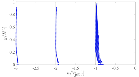
agreement, noting that our dimensionless pressure is defined as , while in [42]it is defined as . The latter results are obtained with artificial viscosity, and artificial diffusion in the continuity equation and energy equation, while in the equation of state an energy term is included. The velocity profiles demonstrate that the collision wall ( ) allows for free-slip wall conditions and suppresses wall penetration.
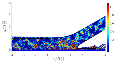
Next, we aim for no-slip wall conditions. In this case the viscosity of the ghost particles is equal to that of the fluid particles ( Ns/m2). With standard SPH this can only be achieved by increasing the fluid viscosity to high, artificial values, resulting in low Reynolds numbers and parabolic velocity profiles, typically valid for laminar flows. With the particle collision model however, this can be achieved at a real viscosity―in this case of water―allowing for much higher Reynolds numbers. In Figure 11 the results of an SPH simulation with particle collisions are shown at ( m/s). Due to the no-slip condition a boundary layer arises, so that the particle distribution now slightly deviates from the free-surface contours. At this Reynolds number, the velocity profiles (Figure 11(b)) are no longer parabolic. This is revealed by the presence of a finite and distinct boundary layer, also seen in turbulent flows. With particle collisions it is thus not necessary to increase the viscosity to high artificial values. The no-slip wall condition is satisfied at the real viscosity Ns/m2 of water, even at a high jet velocity.
 (a)
(a)
 (b)
(b)
Figure 10. Jet impinging on wall ( ). SPH simulation with collision wall showing (a) the particle distribution and free surface contours of Milne-Thomson [43](black lines) and dimensionless pressure (color bar) and (b) the dimensionless vertical velocity profiles. (a) Particle distribution; (b) Velocity profiles.
 (a)
(a)
 (b)
(b)
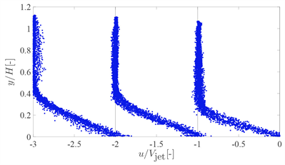
Figure 11. Jet impinging on wall ( ). SPH simulation with particle collisions showing (a) the particle distribution with dimensionless pressure and (b) the dimensionless vertical velocity profiles at horizontal positions and −2. (a) Particle distribution; (b) Velocity profiles.
6. Conclusions
In this paper the use of kinematic conditions rather than dynamic conditions is explored to prevent particle clustering and wall penetration. The kinematic conditions are obtained from kinetic collision theory, which ensures the conservation of momentum and, under certain conditions, conservation of energy as well. This has resulted in the particle collision model, which is based on velocities rather than forces. It is shown that the model acts as a time and space dependent viscosity model, introducing viscosity only when and where it is necessary, thus allowing for real (low laminar) viscosities. As such it may also be used to impose no-slip wall conditions. In addition, the model stabilises the interface between two fluids, and as such may be used as a multi-fluid model in liquid-gas applications with high, realistic density and wave speed ratios.
The particle collision concept is explored in a number of case studies. In all cases the particle collision concept was found to prevent the clustering of particles. The stagnant flow in a reservoir and the dam break flow showed that the method is able to stabilise the interface in typical liquid-gas configurations with density ratios up to 1000:1. It also allows for realistic wave speed ratios and far beyond, which to date could not be achieved within weakly compressible SPH. It is demonstrated that the particle collision model allows for real viscosities, much lower than artificial viscosities.
With standard SPH the no-slip condition can only be satisfied with a high (artificial) viscosity. In that case the velocity profiles show the characteristics of a laminar flow. In the jet flow case it is demonstrated that the particle collision model allows for no-slip conditions with a low (real) viscosity, even at high velocities. In that case the velocity profiles are no longer parabolic and show a finite and distinct boundary layer. It is demonstrated that the collision wall model allows for free slip conditions and may well be used to suppress wall penetration.
It is concluded from the parameter studies in the cases that the best results, with a minimum of dissipation, are obtained with a zero restitution coefficient ( ), while the differences in the range are small. The collision distance is case dependent and can be evaluated from the maximum pressure. The best results are found for .
The particle collision model may be seen as a particle shifting method, in the sense that the velocities are changed, and as a consequence of that the particle positions change. Because it is based on direct changes in velocities rather than forces it allows for a more robust SPH for engineering.
Final Remarks and Future Work
In this work the particle collision concept is applied within weakly compressible SPH; in principle it can also be applied in incompressible SPH. Artificial viscosity has effects similar to a subgrade scale turbulence model [45]. Turbulence is modelled by a smoothed velocity at the scale of the smoothing length [46]. The particle collision model does not rely on a smoothing kernel, so that effectively a (small scale) hat function is used. More investigation is needed in how far turbulent viscosity is or may be represented by the time and space dependent viscosity introduced by inelastic collisions. Also, more investigation is needed in how far the particle collision concept may be used without any dissipation of energy, for example by changing the particle positions due to collisions, but not their velocities.
Acknowledgements
The second author kindly acknowledges support from the Nederlandse Organisatie voor Wetenschappelijk Onderzoek (NWO) VICI Grant 639.033.008. We also thank Andrea Colagrossi for providing the data from [41]used in Section 5.3.
Conflicts of Interest
The authors declare no conflicts of interest regarding the publication of this paper.
Cite this paper
Kruisbrink, A., Korzilius, S., Pearce, F. and Morvan, H. (2018) SPH Particle Collisions for the Reduction of Particle Clustering, Interface Stabilisation and Wall Modelling. Journal of Applied Mathematics and Physics, 6, 1860-1882. https://doi.org/10.4236/jamp.2018.69158
References
- 1. Gingold, R.A. and Monaghan, J.J. (1977) Smoothed Particle Hydrodynamics: Theory and Application to Nonspherical Stars. Monthly Notices of the Royal Astronomical Society, 181, 375-389. https://doi.org/10.1093/mnras/181.3.375
- 2. Lucy, L.B. (1977) A Numerical Approach to the Testing of Fission Hypothesis. The Astronomical Journal, 82, 1013-1024. https://doi.org/10.1086/112164
- 3. Monaghan, J.J. (2012) Smoothed Particle Hydrodynamics and Its Diverse Applications. Annual Review of Fluid Mechanics, 44, 323-346. https://doi.org/10.1146/annurev-fluid-120710-101220
- 4. Price, D.J. (2012) Smoothed Particle Hydrodynamics and Magnetohydrodynamics. Journal of Computational Physics, 231, 759-794. https://doi.org/10.1016/j.jcp.2010.12.011
- 5. Monaghan, J.J. (2000) SPH without a Tensile Instability. Journal of Computational Physics, 159, 290-311. https://doi.org/10.1006/jcph.2000.6439
- 6. Swegle, J.W., Hicks, D.L. and Attaway, S.W. (1995) Smoothed Particle Hydrodynamics Stability Analysis. Journal of Computational Physics, 116, 123-134. https://doi.org/10.1006/jcph.1995.1010
- 7. Monaghan, J.J. and Gingold, R.A. (1983) Shock Simulation by the Particle Method SPH. Journal of Computational Physics, 52, 374-389. https://doi.org/10.1016/0021-9991(83)90036-0
- 8. Monaghan, J.J. and Pongracic, H. (1985) Artificial Viscosity for Particle Methods. Applied Numerical Mathematics, 1, 187-194. https://doi.org/10.1016/0168-9274(85)90015-7
- 9. Balsara, D.S. (1995) Von Neumann Stability Analysis of Smoothed Particle Hydrodynamics—Suggestions for Optimal Algorithms. Journal of Computational Physics, 121, 357-372. https://doi.org/10.1016/S0021-9991(95)90221-X
- 10. Morris, J.P. and Monaghan, J.J. (1997) A Switch to Reduce SPH Viscosity. Journal of Computational Physics, 136, 41-50. https://doi.org/10.1006/jcph.1997.5690
- 11. Cullen, L. and Dehnen, W. (2010) Inviscid Smoothed Particle Hydrodynamics. Monthly Notices of the Royal Astronomical Society, 408, 669-683. https://doi.org/10.1111/j.1365-2966.2010.17158.x
- 12. Chaniotis, A.K., Poulikakos, D. and Koumoutsakos, P. (2002) Remeshed Smoothed Particle Hydrodynamics for the Simulation of Viscous and Heat Conducting OWS. Journal of Computational Physics, 182, 67-90. https://doi.org/10.1006/jcph.2002.7152
- 13. Schussler, M. and Schmitt, D. (1981) Comments on Smoothed Particle Hydrodynamics. Astronomy & Astrophysics, 97, 373-379.
- 14. Johnson, G.R. and Beissel, S.R. (1996) Normalized Smoothing Functions for SPH Impact Computations. International Journal for Numerical Methods in Engineering, 39, 2725-2741. 3.0.CO;2-9>https://doi.org/10.1002/(SICI)1097-0207(19960830)39:16<2725::AID-NME973>3.0.CO;2-9
- 15. Read, J.I., Hayfield, T. and Agertz, O. (2010) Resolving Mixing in Smoothed Particle Hydrodynamics. Monthly Notices of the Royal Astronomical Society, 405, 1513-1530. https://doi.org/10.1111/j.1365-2966.2010.16577.x
- 16. Korzilius, S.P., Kruisbrink, A.C.H., Yue, T., Schilders, W.H.A. and Anthonissen, M.J.H. (2014) Momentum Conserving Methods That Reduce Particle Clustering in SPH. Proceedings of the 9th International SPHERIC Workshop, Paris, 3-5 June 2014, 268-275.
- 17. Dehnen, W. and Aly, H. (2012) Improving Convergence in Smoothed Particle Hydrodynamics Simulations without Pairing Instability. Monthly Notices of the Royal Astronomical Society, 425, 1068-1082. https://doi.org/10.1111/j.1365-2966.2012.21439.x
- 18. Colagrossi, A., Antuono, M., Grenier, N., Le Touze, D. and Molteni, D. (2008) Simulation of Interfacial and Free-Surface Flows Using a New SPH Formulation. Proceedings of the 3rd International SPHERIC Workshop, Lausanne, 4-6 June 2008, 17-23.
- 19. Monaghan, J.J. (2011) A Simple and Efficient SPH Algorithm for Multi-Fluids. Proceedings of the 6th International SPHERIC Workshop, Hamburg, 8-10 June 2011, 172-178.
- 20. Kruisbrink, A., Pearce, F.R., Yue, T., Cliffe, K.A. and Morvan, H.P. (2012) SPH Multi-Fluids Model with Interface Stabilization Based on Quasi-Buoyance Correction. Proceedings of the 7th International SPHERIC Workshop, Prato, 29-31 May 2012, 317-323.
- 21. Kruisbrink, A.C.H., Pearce, F.R., Yue, T. and Morvan, H.P. (2018) An SPH Multi-Fluids Model Based on Quasi Buoyancy for Interface Stabilization up to High Density Ratios and Realistic Wave Speed Ratios. Journal for Numerical Methods in Fluids, 87, 487-507. https://doi.org/10.1002/fld.4498
- 22. Xu, R., Stansby, P. and Laurence, D. (2009) Accuracy and Stability in Incompressible SPH (ISPH) Based on the Projection Method and a New Approach. Journal of Computational Physics, 228, 6703-6725. https://doi.org/10.1016/j.jcp.2009.05.032
- 23. Lind, S.J., Stansby, P.K. and Rogers, B.D. (2016) Incompressible-Compressible Flows with a Transient Discontinuous Interface Using Smoothed Particle Hydrodynamics (SPH). Journal of Computational Physics, 309, 129-147. https://doi.org/10.1016/j.jcp.2015.12.005
- 24. Lind, S.J., Xu, R., Stansby, P.K. and Rogers, B.D. (2012) Incompressible Smoothed Particle Hydrodynamics for Free-Surface Flows: A Generalised Diffusion-Based Algorithm for Stability and Validations for Impulsive Flows and Propagating Waves. Journal of Computational Physics, 231, 1499-1523. https://doi.org/10.1016/j.jcp.2011.10.027
- 25. Kelager, M. (2006) Lagrangian Fluid Dynamics Using Smoothed Particle Hydrodynamics. Master’s Thesis, University of Copenhagen, Copenhagen.
- 26. Meteer, O. (2011) Interaction between SPH Fluids and Dynamics Particle-Based Objects Using CUDA. Proceedings of the 15th Twente Student Conference on IT, Enschede, 20 June 2011.
- 27. Monaghan, J.J. (2005) Smoothed Particle Hydrodynamics. Reports on Progress in Physics, 68, 1703-1759. https://doi.org/10.1088/0034-4885/68/8/R01
- 28. Cleary, P.W. (1998) Modelling Confined Multi-Material Heat and Mass Flows Using SPH. Applied Mathematical Modelling, 22, 981-993. https://doi.org/10.1016/S0307-904X(98)10031-8
- 29. Monaghan, J.J. (1992) Smoothed Particle Hydrodynamics. Annual Review of Astronomy and Astrophysics, 30, 543-574. https://doi.org/10.1146/annurev.aa.30.090192.002551
- 30. Wendland, H. (1995) Piecewise Polynomial, Positive Definite and Compactly Supported Radial Functions of Minimal Degree. Advances in Computational Mathematics, 4, 389-396. https://doi.org/10.1007/BF02123482
- 31. Murnaghan, F.D. (1944) The Compressibility of Media under Extreme Pressures. Proceedings of the National Academy of Sciences of the United States of America, 30, 244-247. https://doi.org/10.1073/pnas.30.9.244
- 32. Gilvarry, J.J. (1957) Temperature-Dependent Equations of State of Solids. Journal of Applied Physics, 28, 1253-1261. https://doi.org/10.1063/1.1722628
- 33. MacDonald, J.R. (1966) Some Simple Isothermal Equations of State. Reviews of Modern Physics, 38, 669-679. https://doi.org/10.1103/RevModPhys.38.669
- 34. Springel, V. (2010) Smoothed Particle Hydrodynamics in Astrophysics. Annual Review of Astronomy and Astrophysics, 48, 391-430. https://doi.org/10.1146/annurev-astro-081309-130914
- 35. Hu, X.Y. and Adams, N.A. (2007) An Incompressible Multi-Phase SPH Method. Journal of Computational Physics, 227, 264-278. https://doi.org/10.1016/j.jcp.2007.07.013
- 36. Hu, X.Y. and Adams, N.A. (2009) A Constant-Density Approach for Incompressible Multi-Phase SPH. Journal of Computational Physics, 228, 2082-2091. https://doi.org/10.1016/j.jcp.2008.11.027
- 37. Colagrossi, A. and Landrini, M. (2003) Numerical Simulation of Interfacial Flows by Smoothed Particle Hydrodynamics. Journal of Computational Physics, 191, 448-475. https://doi.org/10.1016/S0021-9991(03)00324-3
- 38. Monaghan, J.J. (1994) Simulating Free Surface Flows with SPH. Journal of Computational Physics, 110, 399-406. https://doi.org/10.1006/jcph.1994.1034
- 39. Liu, G.R. and Liu, M.B. (2003) Smoothed Particle Hydrodynamics. World Scientific Publishing, Singapore. https://doi.org/10.1142/5340
- 40. Bonet, J. and Rodríguez-Paz, M.X. (2005) Hamiltonian Formulation of the Variable-h SPH Equations. Journal of Computational Physics, 209, 541-558. https://doi.org/10.1016/j.jcp.2005.03.030
- 41. Antuono, M., Colagrossi, A. and Marrone, S. (2012) Numerical Diffusive Terms in Weakly-Compressible SPH Schemes. Computer Physics Communications, 183, 2570-2580. https://doi.org/10.1016/j.cpc.2012.07.006
- 42. Antuono, M., Colagrossi, A., Marrone, S. and Molteni, D. (2010) Free-Surface Flows Solved by Means of SPH Schemes with Numerical Diffusive Terms. Computer Physics Communications, 181, 532-549. https://doi.org/10.1016/j.cpc.2009.11.002
- 43. Milne-Thomson, L.M. (1968) Theoretical Hydrodynamics. 5th Edition, Dover Publications, Mineola. https://doi.org/10.1007/978-1-349-00517-8
- 44. Marrone, S., Antuono, M., Colagrossi, A., Colicchio, G., Le Touzé, D. and Graziani, G. (2011) δ-SPH Model for Simulating Violent Impact Flows. Computer Methods in Applied Mechanics and Engineering, 200, 1526-1542. https://doi.org/10.1016/j.cma.2010.12.016
- 45. Arena, S.E., Gonzalez, J.-F. and Crespe, E. (2011) Characterisation of SPH Noise in Simulations of Protoplanetary Discs. The Astrophysics of Planetary Systems: Formation, Structure, and Dynamical Evolution, 6, 393-394.
- 46. Monaghan, J.J. (2011) A Turbulence Model for Smoothed Particle Hydrodynamics. European Journal of Mechanics B Fluids, 30, 360-370. https://doi.org/10.1016/j.euromechflu.2011.04.002