ABSTRACT

To understand any statistical tool requires not only an understanding of the relevant computational procedures but also an awareness of the assumptions upon which the procedures are based, and the effects of violations of these assumptions. In our earlier articles (Laverty, Miket, & Kelly [1] ) and (Laverty & Kelly, [2] [3] ) we used Microsoft Excel to simulate both a Hidden Markov model and heteroskedastic models showing different realizations of these models and the performance of the techniques for identifying the underlying hidden states using simulated data. The advantage of using Excel is that the simulations are regenerated when the spreadsheet is recalculated allowing the user to observe the performance of the statistical technique under different realizations of the data. In this article we will show how to use Excel to generate data from a one-way ANOVA (Analysis of Variance) model and how the statistical methods behave both when the fundamental assumptions of the model hold and when these assumptions are violated. The purpose of this article is to provide tools for individuals to gain an intuitive understanding of these violations using this readily available program.

Keywords:

Excel, One-Way ANOVA, Assumption Violations, t-Distribution, Cauchy Distribution

1. Introduction

An important aspect of any statistical procedure is the assumptions that the procedure is based on. For example, using the t-distribution to calculate a 95% confidence interval for the centre of the population that is being sampled requires that the population being sampled is a normal distribution and that the observations in the sample are independent. If these underlying assumptions do not hold, the desired performance of the statistical procedure may no longer hold true. Sometimes the effect of an invalid assumption on a property of the procedure is minimal, sometimes not so. If the population is non-normal but has a finite mean and variance (such that the Law of Large Numbers and the Central Limit theorem applies), the departure from normality will have little effect on the properties of confidence intervals computed assuming normality when the sample size is adequately large. The reason for this is that it is a consequence of the Central Limit Theorem. The purpose of this paper is to show how to use the program Excel to simulate data for which the statistical technique of one-way Analysis of Variance (ANOVA) is used. The advantage of the using the program Excel is that when you press the recalculate button, under the Formulas menu, the data that is generated at random will be regenerated, statistical calculations will be recalculated and relevant graphs will be redrawn. This allows the user to observe the variation in these procedures for different realizations of the data. See Figure 1.

2. A Model for Non-Normality (The Cauchy Distribution, the t-Distribution)

For most cases when one-way ANOVA is applicable the normality assumption is appropriate, i.e. the departures of individual observations from their central value are normally distributed. There are however, many examples where this is not the case and extreme departures are more prevalent than predicted by the Normal distribution. This would be dependent on the measurements being collected. For example, if the measurements were measurements of blood pressure, IQ, performance of a political leader one may expect the presence of extreme measurements. In such cases an appropriate model of the departures from the central value would be the t-distribution (a heavy tailed distribution). In this article the reader can use the technique provided to explore the effects of sampling from heavy tailed distributions on ANOVA calculations that assume normality.

The probability density function of the standard Normal, Students t-distribution with ν degrees of freedom and the standard Cauchy distribution is given in (1).

$\begin{array}{l}{f}_{\text{Normal}}\left(z\right)=\frac{1}{\sqrt{2\pi }}{\text{e}}^{-z^2}\\ f_t\left(t:\nu \right)=\frac{\Gamma \left(\frac{\nu +1}{2}\right)}{\sqrt{\nu \pi }\Gamma \left(\frac{\nu }{2}\right)}{\left(1+\frac{t^2}{\nu }\right)}^{-\frac{\nu +1}{2}}\\ f_{\text{Cauchy}}\left(x:0,1\right)=\frac{1}{\pi \left(1+x^2\right)}\end{array}\}$ (1)

The Standard Cauchy distribution is equivalent to the t distribution with 1 degree of freedom. A graph of the standard normal distribution, the t-distribution with 5 degrees of freedom, and the Cauchy distribution is in Figure 2.

The Cauchy Distribution is an example of a distribution where the Law of Large numbers and the Central limit Theorem do not apply [4] . In order for these two Laws to hold both the mean and higher moments have to exist and be finite. This is not the case for the Cauchy distribution. There is no convergence of the distribution of the sample mean to the central value. In fact the distribution of the sample mean is the Cauchy distribution for any sample size (i.e. the distribution of the sample mean is the same as that of any individual observation when the data comes from the Cauchy distribution). The Cauchy distribution is a heavy-tailed distribution. The t-distribution is also a heavy-tailed distribution (but not as extreme) when the degrees of freedom ν is small. As the degrees of freedom increases the t distribution approaches the standard normal distribution. Tsay [5] uses the t-distribution with 5 degrees to model random disturbances that appear in various time series models of financial data. This accounts for the sometimes extreme changes that appear in financial data. The Cauchy distribution is appropriate if extreme values are prevalent in the data (the t-distribution with degrees of freedom higher than 1 in the less extreme case). This could occur in surveys where individuals were asked to make a continuous measurement of some quantity and extreme values were prevalent in the populations. For example, measurements of blood pressure, IQ, and performance of a political leader, could result in non-normal data with extreme values at either end. In such cases alternatives to ANOVA are appropriate.1 We haven’t considered these alternatives in this paper.

The t-distribution with ν degrees of freedom can also be shown to be mixture of Normal distributions with mean 0 and variance W, where the weighting distribution for W is the inverse gamma distribution with α = ν/2 and β = ν/2 (Cook [6] ). This implies that a random variable T will have the t-distribution with ν degrees of freedom if W is selected from the inverse gamma distribution with α = ν/2 and β = ν/2 and then T is selected from Normal distributions with mean 0 and variance W.

3. Simulation of Data from a Continuous Distribution in Excel

Uniform random variates on [0,1] can be generated in Excel with the function “RAND()”. The generation of random variates from a continuous distribution with measure of central location μ and measure of scale σ, can be carried out using the inverse-transform method (Fishman [7] ). Namely Y = F⁻¹⁽U) where F(u) is the desired cumulative distribution of Y and U has a uniform distribution on [0,1] (seeFigure 3). In Excel this is achieved for the Normal distribution (mean μ, standard deviation σ) with the function “μ+σ*NORMSINV(RAND())” and for the Cauchy (t with 1 d.f.) location parameter, μ, and scale parameter, σ, “μ+σ*TINV(2*(1-RAND()),1)” (Figure 3).

Comment:The Excel function TINV(U,df) does not calculate F⁻¹(U) for the t-distn with degrees of freedom df, however the excel function TINV(2*(1-U),df) does achieve the desired calculation.

4. Setting Up the Excel Worksheet to Simulate Anova Data

The data simulated will come from 3 populations (this can easily be generalized to more than 3 populations). The parameters of the populations

1) mean(central location), stored in cells C2:E2

2) standarddeviation (scale parameter), stored in cells C3:E3

3) samplesize), stored in cells C4:E4

4) aparameter that determines normality of the data versus non-normality. stored in cells C1:E1. This parameter is set to zero if the desired data is normal. If this parameter is set to an integer, ν, greater than 0 the data will come from a t -distribution with ν degrees of freedom. The t -distribution is a non-normal heavy-tailed, centered and symmetric about zero.

5) A final parameter (precision), located in cell A2 specifies the of decimal places that the raw data is rounded to (Table 1 below)

5. Generating Simulated Data

Copy the observation numbers (1 to 10) in Cells B7:B:16

Paste in cell C7 the formula =IF($B7>C$4,"",ROUND(C$2+C$3*IF(C$1=0,NORMSINV(RAND()),TINV(2*(1-RAND()),C$1)),$A$2))”

Copy this formula to cells C7:E16. If the normality parameter is 0, the data generated will be from the normal distribution with mean = “loc. Par.” And standard deviation = “scale par.”). If the normality parameter is an integer greater than 0, the data will be a random number with a t-distribution scaled by the “scale par.” and location shifted by the “loc. par.” The data will be rounded to the number of decimals specified by “precision”.

For each population compute T_i = Sxand Sx². Paste formula “=SUM(C7:C16)” and formula “=SUMSQ(C7:C16)” in cells C18 and C19. Copy these formulae to cells C18:E19.

6. Computation of Statistics Required for One-Way ANOVA

Suppose we have data from k Normal populations with means ${\mu }_{\text{1}},{\mu }_{\text{2}},{\mu }_{\text{3}},\cdots ,{\mu }_k$ and common standard deviation σ.Let $\left\{x_{ij},i=\text{1},\text{2},\cdots ,k;j=\text{1},\text{2},\cdots ,n_i\right\}$ denote data from these populations. Let x_ij = the j^th observation from the i^th population, n_i = the sample size from the i^th population.

Let

${\overline{x}}_i=\frac{{\displaystyle {\sum }_{j=1}^{n_i}{x}_{ij}}}{n_i}$ and $s_i=\sqrt{\frac{{\displaystyle {\sum }_{j=1}^{n_i}{\left(x_{ij}-{\overline{x}}_i\right)}^2}}{n_i-1}}$ (2)

denotethe sample mean and standard deviation from the i^th population. To compute the sample mean and sample Standard deviation for each population, paste the formulae “=AVERAGE(C7:C16)”and “=STDEV(C7:C16)”in cells C21 and C22. Copy these formulae to cells C21:E22.

To test the null hypothesis H₀: ${\mu }_{\text{1}}={\mu }_{\text{2}}=\cdots ={\mu }_k$ against H_A: ${\mu }_i\ne {\mu }_j$ for at least one pair i, j we use the test statistic

$F=\frac{{\displaystyle {\sum }_{i=1}^k{\left({\overline{x}}_i-{\overline{x}}_{.}\right)}^2/\left(k-1\right)}}{{\displaystyle {\sum }_{i=1}^k{\displaystyle {\sum }_{j=1}^{n_i}{\left(x_{ij}-{\overline{x}}_i\right)}^2/\left(N-k\right)}}}=\frac{{\text{SS}}_{\text{Between}}/\left(k-1\right)}{{\text{SS}}_{\text{Within}}/\left(N-k\right)}$ . (3)

where

${\text{SS}}_{\text{Between}}={\displaystyle {\sum }_{i=1}^k{\left({\overline{x}}_i-{\overline{x}}_{.}\right)}^2}$ and ${\text{SS}}_{\text{Within}}={\displaystyle {\sum }_{i=1}^k{\displaystyle {\sum }_{j=1}^{n_i}{\left(x_{ij}-{\overline{x}}_i\right)}^2}}$ (4)

This statistic has an F-distribution with ν₁ = k – 1 degrees of freedom in the numerator and ν₂ = N – k degrees of freedom in the denominator.

The computing formulae for

${\text{SS}}_{\text{Between}}={\displaystyle {\sum }_i\frac{T_i^2}{n_i}}-\frac{G^2}{N}$ and ${\text{SS}}_{\text{Within}}={\displaystyle {\sum }_i{\displaystyle {\sum }_j{x}_{ij}^2}}-{\displaystyle {\sum }_i\frac{T_i^2}{n_i}}$ (5)

where

$T_i={\displaystyle {\sum }_i{x}_{ij}}={\displaystyle \sum {\displaystyle \sum x_{ij}}}$ and $G={\displaystyle {\sum }_i{T}_i}={\displaystyle \sum {\displaystyle \sum x_{ij}}}$ (6)

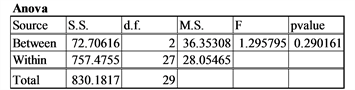
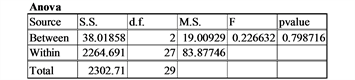
The testing for One-way ANOVA is carried out using the Analysis of Variance table (Table 2).

Place the formula “=SUM(C18:E18)” in cell G18 to compute the grand total, $G={\displaystyle {\sum }_i{T}_i}={\displaystyle \sum {\displaystyle \sum x_{ij}}}$ and the formula “=SUM(C19:E19)” in cell G19 to compute ${\displaystyle \sum {\displaystyle \sum x_{ij}^2}}.$

Place the formula “=C18²/C4” in cell C24 and copy to E24 to compute $\frac{T_i^2}{n_i}$ for each sample. Then place the formula “=SUM(C24:E24)” in cell G24 to compute ${\displaystyle {\sum }_i\frac{T_i^2}{n_i}}$ .

To compute ${\text{SS}}_{\text{Between}}={\displaystyle {\sum }_i\frac{T_i^2}{n_i}}-\frac{G^2}{N}$ place the formula “=G24-G18²/F4” in cell J22 and to compute ${\text{SS}}_{\text{Within}}={\displaystyle {\sum }_i{\displaystyle {\sum }_j{x}_{ij}^2}}-{\displaystyle {\sum }_i\frac{T_i^2}{n_i}}$ place the formula = G19-G24” in J23.

The formulae for degrees of freedom, Mean Square can be placed in the appropriate cells L22:L23 and K22:K23.

The formula for the F statistic “=L22/L23” can be placed in cell M22. The formula for the p-value of the observed F value “=FDIST(M22, K22,K23)” can be placed in cell N22.

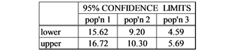
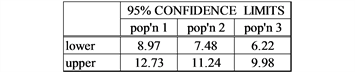
The formula for a (1−α)100% confidence interval for the mean of the ith sample is:

${\overline{x}}_i\pm t_{\alpha /2}^{\left(d{f}_{\text{Error}}\right)}\frac{\sqrt{{\text{MS}}_{\text{Error}}}}{n_i}$ (7)

This formula “=C$21-TINV(0.05,$K$23)*(SQRT($L$23)/$C$4)” can be placed in Cell I28 for the lower limit and in cell I29 “=C$21+TINV(0.05,$K$23)*(SQRT($L$23)/$C$4)” for the upper limit. These formulae can be copied to cells I28:K29 to do the computation for all samples.

The spreadsheet should now look like Figure 4.

To construct Box-whisker plots of the data

1) Select a range containing the data C6:E16 for 10 observations from each sample from the 3 Populations.

2) The menu item for Box-plots can be found under the histogram item (Figure 5).

Comment: There is a problem with Excel’s method of drawing box-plots. If in the data range there is a blank cell, when drawing a box-plot Excel treats that cell as containing a zero rather than treating the observation as non-existent.

7. Exercises That Can Be Performed to Illustrate the Effects of Assumption Violations on ANOVA

In these exercises we generate samples using different ANOVA assumptions to examine the violations of these assumptions on the ANOVA calculations.

1) Equal means, Equal Standard deviations, Equal sample size, Normality:

μ₁= 10, σ₁ = 2, n₁ = 10,μ₂= 10, σ₂ = 2, n₂ = 10, μ₃ = 10, σ₃ = 2, n₃ = 10; normality = 0 (normal distribution)

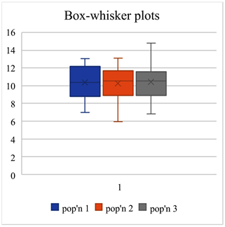
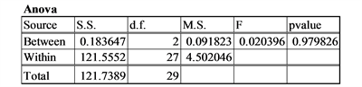
Comment: When the population means are all equal and the assumptions are satisfied the p-values come from a uniform distribution from 0 to 1. Thus 5% of the time the p-value will be less than or equal to 0.05 resulting in a type I error.

2) Unequal means (H₀ false), Equal Standard deviations, Equal sample size, Normality:

μ₁= 15, σ₁ = 2, n₁ = 10,μ₂= 10, σ₂ = 2, n₂ = 10, μ₃ = 5, σ₃ = 2, n₃ = 10; normality = 0 (normal distribution)

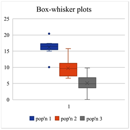
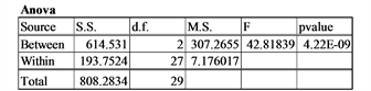
Comment: The ability to detect differences among the means will depend on the non-centralityparameter $\delta =\frac{{\displaystyle {\sum }_i{n}_i{\left({\mu }_i-\mu \right)}^2}}{{\sigma }^2}$ where $\mu =\frac{{\displaystyle {\sum }_i{n}_i{\mu }_i}}{{\displaystyle {\sum }_i{n}_i}}$ .

(Kirk, [8] ) The larger the value of the non-centrality parameter, δ, the greater the power of the F-test. (i.e. the greater the probability of picking out existent differences.)

3) Unequal means (H₀ false), Equal Standard deviations, Equal sample size, Normality (low non-centrality parameter):

μ₁= 11, σ₁ = 5, n₁ = 10,μ₂= 10, σ₂ = 5, n₂ = 10, μ₃ = 9, σ₃ = 5, n₃ = 10; normality = 0 (normal distribution)

Comment: In this case the non-centrality parameter is smaller than the previous example. The p-value of the F-test is considerably higher resulting in an inability to detect a difference in the means.

4) Equal means, Unequal Standard deviations, Equal sample size, Normality:

μ₁= 10, σ₁ = 2, n₁ = 10,μ₂= 10, σ₂ = 5, n₂ = 10, μ₃ = 10, σ₃ = 10, n₃ = 10; normality = 0 (normal distribution))

Comment: The anova F-test is to some extent robust against the violation of the assumption of the homogeneity of variance (Bathke [9] ).

5) Equal means, Equal Standard deviations, Equal sample size, non-Normality:

μ₁= 10, σ₁ = 2, n₁ = 10,μ₂= 10, σ₂ = 2, n₂ = 10, μ₃ = 10, σ₃ = 2, n₃ = 10; normality = 1 (Cauchy distribution)

Comment: Recall when the data comes from the Cauchy distribution (t-distribution 1 d.f.) neither the law of large numbers or the Central Limit Theorem are applicable. In fact, the distribution of the sample mean for n observations is the same as a single observation. This is illustrated in this example.

8. Discussion

In applying any statistical procedure it is important understanding the assumptions on which it is based. It is also important to understand the effects on these procedures of the violations of these assumptions. Sometimes the effects of the violations can be extreme, sometimes minimal. The purpose of this article is to provide tools for individuals to gain an intuitive understanding of these violations using the readily available program Microsoft Excel. The advantage of the using the program Excel is that when you press the recalculate button, under the Formulas menu, the data that is generated at random will be regenerated, statistical calculations will be recalculated and relevant graphs will be redrawn. The statistical procedure that we have chosen to illustrate these tools is one-way ANOVA. This procedure is an important component of introductory statistical courses and textbooks. The tools can be easily extended to other and more advanced univariate procedures.

9. Conclusion

Excel is a very useful tool for examining the performance of One-Way Anova of variance both when the assumptions hold and more importantly when the assumptions are violated.

Conflicts of Interest

The authors declare no conflicts of interest regarding the publication of this paper.

Cite this paper

Laverty, W. and Kelly, I. (2019) Using Excel to Explore the Effects of Assumption Violations on One-Way Analysis of Variance (ANOVA) Statistical Procedures. Open Journal of Statistics, 9, 458-469. https://doi.org/10.4236/ojs.2019.94031

References

NOTES

¹For example, the non-parametric (Kruskal-Wallis).

References

- 1. Laverty, W.H., Miket, M.J. and Kelly, I.W. (2002) Simulation of Hidden Markov Models with EXCEL. Journal of Royal Statistical Society: Series D, 51, 31-40. https://doi.org/10.1111/1467-9884.00296
- 2. Laverty, W.H. and Kelly, I.W. (2018) Using Excel to Simulate and Visualize Conditional Heteroskedastic Models. American Journal of Theoretical and Applied Statistics, 7, 242-246.
- 3. Laverty, W.H. and Kelly, I.W. (2019) Using Excel to Visualize State Identification in Hidden Markov Models Using the Forward and Backward Algorithms. Applied Mathematical Sciences, 13, 151-162. https://doi.org/10.12988/ams.2019.812195
- 4. Feller, W. (1971) An Introduction to Probability Theory and Its Applications, Volume II. 2nd Edition, John Wiley & Sons Inc., New York.
- 5. Tsay, R.S. (2010) Analysis of Financial Time Series. 3rd Edition, Wiley, Hoboken. https://doi.org/10.1002/9780470644560
- 6. Cook, J.D. (2018) Statistical Odds and Ends Blog. https://statisticaloddsandends.wordpress.com/2018/03/03/t-distribution-as-a-mixture-of-normals/
- 7. Fishman, G.S. (1995) Monte Carlo, Concepts, Algorithms and Applications. Springer, Berlin.
- 8. Kirk, R. (2012) Experimental Design: Procedures for Behavioral Sciences. Sage Publications, Thousand Oaks. https://doi.org/10.4135/9781483384733
- 9. Bathke, A. (2004) The Anova F Test Can Still Be Used in Some Balanced Designs with Unequal Variances and Non-normal Data. Journal of Statistical Planning and Inference, 126, 413-422. https://doi.org/10.1016/j.jspi.2003.09.010
NOTES
1For example, the non-parametric (Kruskal-Wallis).