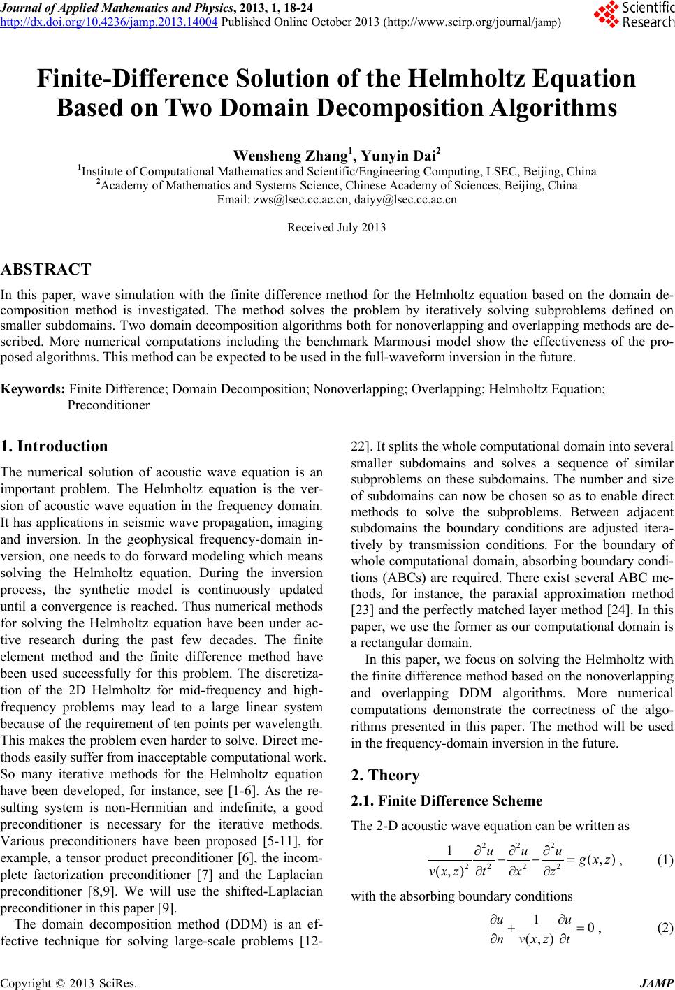
Journal of Applied Mathematics and Physics, 2013, 1, 18-24
http://dx.doi.org/10.4236/jamp.2013.14004 Published Online October 2013 (http://www.scirp.org/journal/jamp)
Finite-Difference Solution of the Helmholtz Equation
Based on Two Domain Decomposition Algorithms
Wensheng Zhang1, Yunyin Dai2
1Institute of Computational Mathematics and Scientific/Engineering Computing, LSEC, Beijing, China
2Academy of Mathematics and Systems Science, Chinese Academy of Sciences, Beijing, China
Received July 2013
ABSTRACT
In this paper, wave simulation with the finite difference method for the Helmholtz equation based on the domain de-
composition method is investigated. The method solves the problem by iteratively solving subproblems defined on
smaller subdomains. T wo domain decomposition algorithms both for nonoverlapping and overlapping methods are de-
scribed. More numerical computations including the benchmark Marmousi model show the effectiveness of the pro-
posed algorithms. This method can be expected to be used in the full-waveform inversion in the future.
Keywords: Finite Difference; Domain Decomposition; Nonoverlapping; Overlapping; Helmholtz Equation;
Preconditioner
1. Introduction
The numerical solution of acoustic wave equation is an
important problem. The Helmholtz equation is the ver-
sion of acoustic wave equation in the frequency domain.
It has applications in seismic wave propagation, imaging
and inversion. In the geophysical frequency-domain in-
version, one needs to do forward modeling which means
solving the Helmholtz equation. During the inversion
process, the synthetic model is continuously updated
until a convergence is reached. Thus numerical methods
for solving the Helmholtz equation have been under ac-
tive research during the past few decades. The finite
element method and the finite difference method have
been used successfully for this problem. The discretiza-
tion of the 2D Helmholtz for mid-frequency and high-
frequency problems may lead to a large linear system
because of the requirement of ten points per wavelength.
This makes the problem even harder to solve. Direct me-
thods easily suffer from inacceptable computational work.
So many iterative methods for the Helmholtz equation
have been developed, f or instance, see [1-6]. As the re-
sulting system is non-Hermitian and indefinite, a good
preconditioner is necessary for the iterative methods.
Various preconditioners have been proposed [5-11], for
example, a tensor product preconditioner [6], the incom-
plete factorization preconditioner [7] and the Laplacian
preconditioner [8,9]. We will use the shifted-Laplacian
precondi tioner i n t hi s paper [9 ] .
The domain decomposition method (DDM) is an ef-
fective technique for solving large-scale problems [ 12-
22]. It splits the whole computational domain into several
smaller subdomains and solves a sequence of similar
subproblems on these subdomains. The number and size
of subdomains can now be chosen so as to enable direct
methods to solve the subproblems. Between adjacent
subdomains the boundary conditions are adjusted itera-
tively by transmission conditions. For the boundary of
whole computational domain, absorbing boundary condi-
tions (ABCs) are required. There exist several ABC me-
thods, for instance, the paraxial approximation method
[23] and the perfectly matched layer method [24]. In this
paper, we use the former as our computational domain is
a rectangular domain.
In this paper, we focus on solving the Helmholtz with
the finite difference method based on the nonoverlapping
and overlapping DDM algorithms. More numerical
computations demonstrate the correctness of the algo-
rithms presented in this paper. The method will be used
in the frequency -domain inversion in the future.
2. Theory
2.1. Finite Difference Scheme
The 2-D acoustic wave equation can be written as
222
222 2
1(,)
(,)
uuu
gxz
vxz txz
∂∂∂
−−=
∂∂∂
, (1)
with the absorbing bounda ry c ondition s
1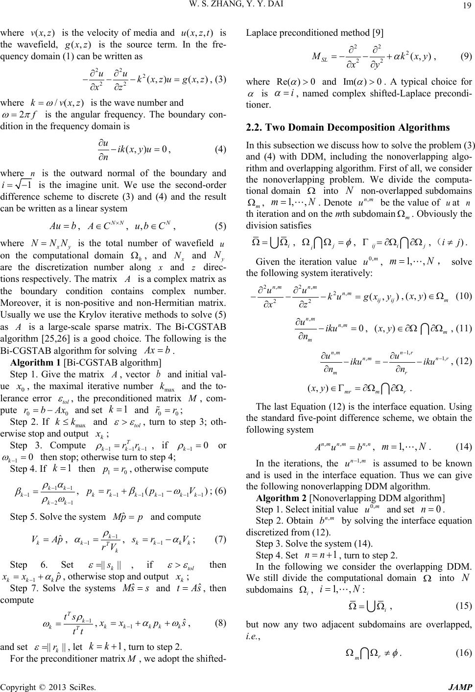0
(,)
uu
n vxzt
∂∂
+=
∂∂
, (2)

W. S. ZHANG, Y. Y. DAI
19
where
(,)vxz
is the velocity of media and
(,,)uxzt
is
the wavefield,
(,)gxz
is the source term. In the fre-
quency domain (1) can be written as
222
22
(,) (,)
uu
k xzugxz
xz
∂∂
−−− =
∂∂
, (3)
where
/(,)k vxz ω =
is the wave number and
2f ωπ =
is the angular frequency. The boundary con-
dition in the frequency domain is
(, )0
uikxy u
n
∂−=
∂
, (4)
where
n
is the outward normal of the boundary and
1i= −
is the imagine unit. We use the second-order
difference scheme to discrete (3) and (4) and the result
can be written as a linear system
Au b=
,
NN
AC
×
∈
,
,N ub C∈
, (5)
where
xy
N NN=
is the total number of wavefield
u
on the computational domain h Ω
, and x
N
and
y
N
are the discretization number along
x
and
z
direc-
tions respectively. The matrix
A
is a complex matrix as
the boundary condition contains complex number.
Moreover, it is non-positive and non-Hermitian matrix.
Usually we use the Krylov iterative methods to solve (5)
as
A
is a large-scale sparse matrix. The Bi-CGSTAB
algorithm [25,26] is a good choice. The following is the
Bi-CGSTAB algorithm for solving
Ax b=
.
Algorithm 1 [Bi-CGSTAB algorithm]
Step 1. Give the matrix
A
, vector
b
and initial val-
ue
0
x
, the maximal iterative number
max
k
and the to-
lerance error tol ε
, the preconditioned matrix
M
, com-
pute
00
rb Ax= −
and set
1k=
and
00
rr=

;
Step 2. If
max
kk≤
and
tol
εε >
, turn to step 3; oth-
erwise st op and out put
k
x
;
Step 3. Compute
1 11
T
k kk
rr ρ
− −−
=
, if
1
0
k
ρ
−
=
or
1
0
k
ω
−
=
then stop; otherwise turn to step 4;
Step 4. If
1k=
then
10
pr=
, otherwi s e c ompute
11
121
kk
kkk
ρα
βρω
−−
−
−−
=
,
11 111
()
k kkkkk
prp V βω
−− −−−
=+−
; (6)
Step 5. Solve the system
ˆ
Mp p=
and compute
ˆ
k
V Ap=
,
1
1k kTk
rV
ρ
α
−
−
=
,
1k kkk
sr V α
−
= −
; (7)
Step 6. Set
|| ||
k
s ε =
, if
tol
εε >
then
1
ˆ
kk k
xx p α
−
= +
, otherwise stop and output
k
x
;
Step 7. Solve the systems
ˆ
Ms s=
and
ˆ
t As=
, then
compute
1
Tk
kT
ts
tt
ρ
ω
−
=
,
1
ˆ
k kkk k
xxp s αω
−
=++
, (8)
and set
|| ||
k
r ε =
, let
1kk= +
, turn to step 2.
For the preconditioner matrix
M
, we adopt the shifted-
Laplace pre conditioned method [9]
22 2
22
(, )
SL
Mk xy
xy
α
∂∂
=−−+
∂∂
, (9)
where
Re( )0 α >
and
Im( )0 α >
. A typical choice for
α
is
i α =
, named complex shifted-Laplace precondi-
tioner.
2.2. Two Domain Decomposition Algorithms
In this subsection we discuss how to s olve the problem (3)
and (4) with DDM, including the nonoverlapping algo-
rithm and overlapping algorithm. First of all, we consider
the nonoverlapping problem. We divide the computa-
tional domain
Ω
into
N
non-overlapped subdomains
m
Ω
,
1, ,mN=
. Denote
,nm
u
be the value of
u
at
n
th iteration and on the mth subdomain
m
Ω
. Obviously the
division satisfies
i
Ω= Ω

,
j
i
φ Ω Ω=

,
ij ij
Γ= ∂Ω∂Ω

,
)ij≠（
.
Given the iteration value
0,m
u
,
1, ,mN=
， solve
the following system iteratively:
2,2, 2,
22
(,)
nmnm nm ij ij
uu
kugx y
xz
∂∂
−−−=
∂∂
,
(, )
m
xy∈Ω
(10)
,,
0
nm nm
m
uiku
n
∂−=
∂
,
(,)
m
xy∈ ∂Ω∂Ω

, (11)
, 1,
, 1,
nmn r
nmn r
mr
uu
iku iku
nn
−−
∂∂
−=− −
∂∂
, (12)
(,)
mrm r
xy∈ Γ=∂Ω∂Ω

.
The last Equation (12 ) is the interface equation. Using
the standard five-point difference scheme, we obtain the
following system
,, ,nm nmnn
Au b=
,
1, ,mN=
. (14)
In the iterations, the
1,nm
u
−
is assumed to be known
and is used in the interface equation. Thus we can give
the following nonoverlapping DDM algorithm.
Algorithm 2 [Nonoverlapping DDM algorithm]
Step 1. Select initial value
0,m
u
and set
0n=
.
Step 2. Obtain
,nm
b
by solving the interface equation
discretized from (12).
Step 3. Solve the system (14).
Step 4. Set
1nn=+
, turn to step 2.
In the following we consider the overlapping DDM.
We still divide the computational domain
Ω
into
N
subdomains
i
Ω
,
1, ,iN=
:
i
Ω= Ω

, (15 )
but now any two adjacent subdomains are overlapped,
i.e.,
r
m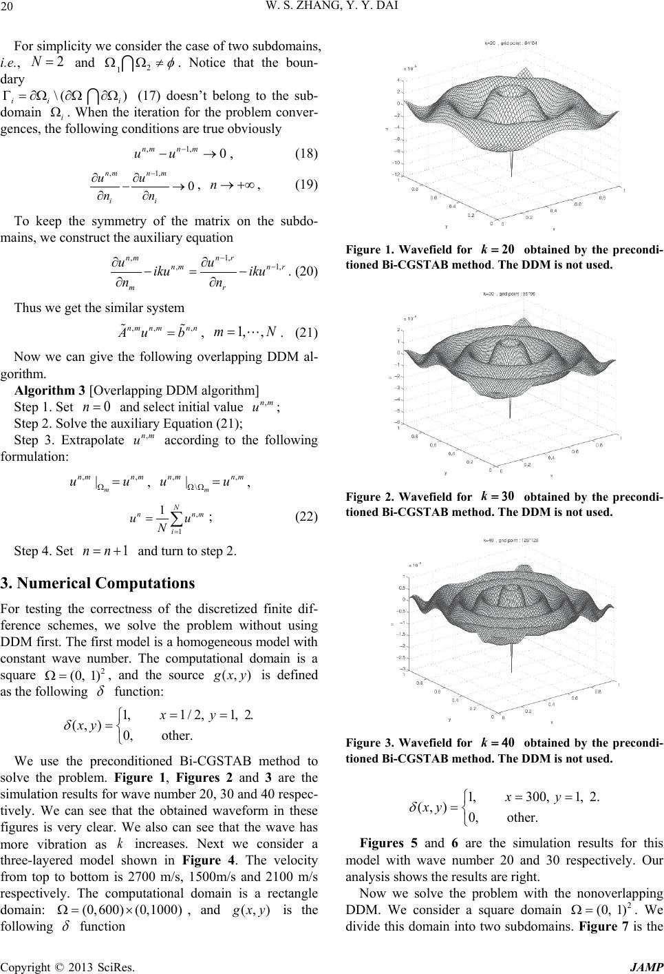
φ Ω Ω≠

. (16 )

W. S. ZHANG, Y. Y. DAI
20
For simplicity we consider the case of two subdomains,
i.e.,
2N=
and
2
1
φ Ω Ω≠

. Notice that the boun-
dary
\( )
ii i
Γ= ∂Ω∂Ω∂Ω

(17) doesn’t belong to the sub-
domain
i
Ω
. When the iteration for the problem conver-
gences, the following conditions are true obviously
, 1,
0
nmn m
uu
−
−→
, (18)
,1, 0 nmn m
ii
uu
nn
−
∂∂
−→
∂∂
,
n→+∞
, (19)
To keep the symmetry of the matrix on the subdo-
mains, we construct the auxiliary equation
, 1,
, 1,
nmn r
nmn r
mr
uu
iku iku
nn
−−
∂∂
−= −
∂∂
. (20)
Thus we get the similar system
,, ,nm nmnn
Au b=

,
1, ,mN=
. (21)
Now we can give the following overlapping DDM al-
gorithm.
Algorithm 3 [Overlapping DDM algorithm]
Step 1. Set
0n=
and select initial value
,nm
u
;
Step 2. Solve the auxiliary Equation (21);
Step 3. Extrapolate
,nm
u
according to the following
formulation:
,,
|m
nm nm
uu
Ω
=
,
,,
\
|m
nm nm
uu
ΩΩ
=
,
,
1
1N
n nm
i
uu
N=
=
∑
; (22)
Step 4. Set
1nn=+
and turn to step 2.
3. Numerical Computations
For testing the correctness of the discretized finite dif-
ference schemes, we solve the problem without using
DDM first. The first model is a homogeneous model with
constant wave number. The computational domain is a
square
2
(0, 1)Ω=
, and the source
(, )gxy
is defined
as the following
δ
function:
1,1/2 , 1, 2.
(, )0, other.
xy
xy δ
= =

=

We use the preconditioned Bi-CGSTAB method to
solve the problem. Figure 1, Figures 2 and 3 are the
simulation results for wav e number 20, 30 and 40 resp ec-
tively. We can see that the obtained waveform in these
figures is very clear. We also can see that the wave has
more vibration as
k
increases. Next we consider a
three-layered model shown in Figure 4. The velocity
from top to bottom is 2700 m/s, 1500m/s and 2100 m/s
respectively. The computational domain is a rectangle
domain:
(0,600) (0,1000)Ω= ×
, and
(, )gxy
is the
following
δ
function
Figure 1. Wavefield for
k20=
obtained by the precondi-
tioned Bi-CGSTAB method. The DDM is not used.
Figure 2. Wavefield for
k0= 3
obtained by the precondi-
tioned Bi-CGSTAB method. The DDM is not used.
Figure 3. Wavefield for
k0= 4
obtained by the precondi-
tioned Bi-CGSTAB m ethod. The DDM is not used.
1,300, 1, 2.
(, )0, other.
xy
xy δ
= =

=

Figures 5 and 6 are the simulation results for this
model with wave number 20 and 30 respectively. Our
analysis shows the results are right.
Now we solve the problem with the nonoverlapping
DDM. We consider a square domain
2
(0, 1)Ω=
. We
divide this domain into two subdomains. Figure 7 is the

W. S. ZHANG, Y. Y. DAI
21
Figure 4. A three-layered model with velocity 2700 m/s,
1500 m/s and 2100 m/s from top to bottom.
Figure 5. Wavefield contour for
f0= 2
Hz obtained by
the preconditioned Bi-CGSTAB method. The DDM is not
used.
Figure 6. Wavefield contour
f30=
Hz obtained by the
preconditioned Bi-CGSTAB m ethod. The DDM i s not used.
wavefield result for f = 4 Hz obtained by the nonoverlap-
ping DDM algorithm with two subdomains. For a L-type
model we divide it into three subdomains. Figure 8 is the
corresponding simulation result for f = 4 Hz obtained by
the nonoverlapping DDM algorithm with three subdo-
mains. Figure 9 is result for f = 4 Hz obtained by the
nonoverlapping DDM method with four equal square
subdomains for a square domain.
Next we solve the problem with the overlapping DDM
algorithm. The velocity media is 2100 m/s. The location
of the pulse is at
(,)(3, 2.5)xy=
. The frequency is
Figure 7. Wavefield for f = 4 Hz obtained by the nonover-
lapping DDM algorithm. The square computational domain
is divided i nt o two subdomains up and down.
Figure 8. Wavefield for f = 4 Hz obtained by the nonover-
lapping DDM algorithm. The L-type computational domain
is divided i nt o thr ee square subdomains.
Figure 9. Wavefield for f = 4 Hz obtained by the nonover-
lapping DDM algor ithm. The square computational domain
is divided i nt o four equal square s ubdomains.

W. S. ZHANG, Y. Y. DAI
22
f = 1 Hz. Figure 10 is the wavefield obtained by the
overlapping DDM algorithm with two equal square sub-
domains up and down. Figure 11 is the wavefield ob-
tained by the overlapping DDM algorithm with three
square subdomains for an L-type domain. Figure 12 is the
Figure 10. Wavefield for f = 1 Hz obtained by the overlap-
ping DDM algorithm. The computational domain is divided
into two equal subdomains up and down.
Figure 11. Wavefield for f = 1 Hz obtained by the overlap-
ping DDM algorithm. The square computational domain is
divided into t hree equal square subdomains.
Figure 12. Wavefield for f = 1 Hz obtained by the overlap-
ping DDM algorithm. The square computational domain is
divided into f ou r equal subdomains.
wavefield obtained by the overlapping DDM algorithm
with four equal squ a re subdomains for a square domain.
Finally we consider a typical inhomogeneous model
named Marmousi model which is usually used to test the
ability of seismic migration and inversion [27]. The ve-
locity is shown in Figure 13. The velocity varies from
1500 m/s to 5500 m/s. We select a part of this model to
simulate wave propagation. Figure 14 is the wavefield
contour obtained by the preconditioned Bi-CGSTAB
method for
5f=
Hz and the DDM algorithm is not used.
Figure 15 is the wavefield contour obtained by the non-
overlapping DDM algorithm with two subdomains. Fig-
ure 16 is the wavefield contour obtained by the overlap-
ping DDM algorithm with two subdomains. Figure 17 is
the similar result but for
20f=
Hz. Comparing Fig-
ures 15 and 16 with Figure 14, we know that they al-
most the same which are just we expect.
4. Conclusion
The acoustic wave equation in the frequency domain is
solved by the finite difference method based on the do-
main decomposition method. The discritizaiton of the
Figure 13. Marmousi model.
Figure 14. Wavefield contour for f = 5 Hz obtained by the
preconditioned Bi-CGSTAB algorithm. The DDM algo-
rithm is not use d.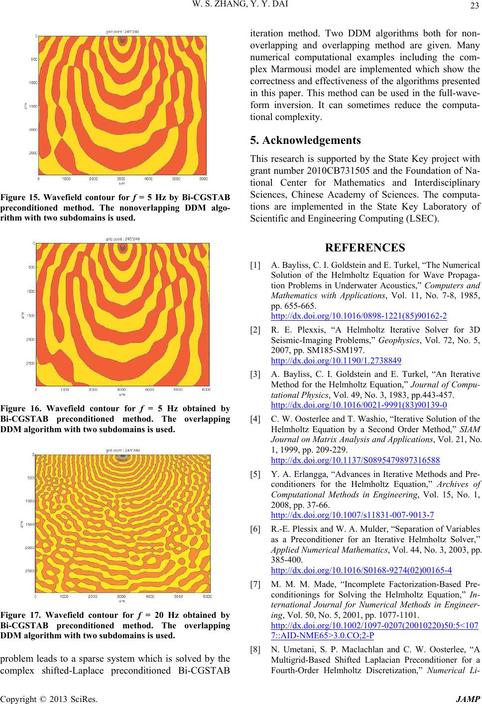

W. S. ZHANG, Y. Y. DAI
23
Figure 15. Wavefield contour for f = 5 Hz by Bi-CGSTAB
preconditioned method. The nonoverlapping DDM algo-
rithm with two subdomains is use d.
Figure 16. Wavefield contour for f = 5 Hz obtained by
Bi-CGSTAB preconditioned method. The overlapping
DDM algorithm with two subdomains is used.
Figure 17. Wavefield contour for f = 20 Hz obtained by
Bi-CGSTAB preconditioned method. The overlapping
DDM algorithm with two subdomains is used.
problem leads to a sparse system which is solved by the
complex shifted-Laplace preconditioned Bi-CGSTAB
iteration method. Two DDM algorithms both for non-
overlapping and overlapping method are given. Many
numerical computational examples including the com-
plex Marmousi model are implemented which show the
correctness and effectiveness of the algorithms presented
in this paper. This method can be used in the full-wave-
form inversion. It can sometimes reduce the computa-
tional complexity.
5. Acknowledgements
This research is supported by the State Key project with
grant number 2010CB73 1505 and the Foundation of N a-
tional Center for Mathematics and Interdisciplinary
Sciences, Chinese Academy of Sciences. The computa-
tions are implemented in the State Key Laboratory of
Scienti f i c an d Engineering Computing (LSEC).
REFERENCES
[1] A. Bayliss, C. I. Goldstein and E. Turkel, “The Numerical
Solution of the Helmholtz Equation for Wave Propaga-
tion Problems in Underwater Acoustics,” Computers and
Mathematics with Applications, Vol. 11, No. 7-8, 1985,
pp. 655-665.
http://dx.doi.org/10.1016/0898-1221(85)90162-2
[2] R. E. Plexxis, “A Helmholtz Iterative Solver for 3D
Seismic-Imaging Problems,” Geophysics, Vol. 72, No. 5,
2007, pp. SM185-SM197.
http://dx.doi.org/10.1190/1.2738849
[3] A. Bayliss, C. I. Goldstein and E. Turkel, “An Iterative
Method for the Helmholtz Equation,” Journal of Compu-
tational Physics, Vol. 49, No. 3, 1983, pp.443-457.
http://dx.doi.org/10.1016/0021-9991(83)90139-0
[4] C. W. Oosterlee and T. Washio, “Iterative Solution of the
Helmholtz Equation by a Second Order Method,” SIAM
Journal on Matrix Analysis and Applications, Vol. 21, No.
1, 1999, pp. 209-229.
http://dx.doi.org/10.1137/S0895479897316588
[5] Y. A. Erlangga, “Advances in Iterative Methods and Pre-
conditioners for the Helmholtz Equation,” Archives of
Computational Methods in Engineering, Vol. 15, No. 1,
2008, pp. 37-66.
http://dx.doi.org/10.1007/s11831-007-9013-7
[6] R.-E. Plessix a nd W. A. Mulder, “Separation of Variables
as a Preconditioner for an Iterative Helmholtz Solver,”
Applied Numerical Mathematics, Vol. 44, No. 3, 2003, pp.
385-400.
http://dx.doi.org/10.1016/S0168-9274(02)00165-4
[7] M. M. M. Made, “Incomplete Factorization-Based Pre-
conditionings for Solving the Helmholtz Equation,” In-
ternational Journal for Numerical Methods in Engineer-
ing, Vol. 50, No. 5, 2001, pp. 1077-1101.
http://dx.doi.org/10.1002/1097-0207(20010220)50:5<107
7::AID-NME65>3.0.CO;2-P
[8] N. Umetani, S. P. Maclachlan and C. W. Oosterlee, “A
Multigrid-Based Shifted Laplacian Preconditioner for a
Fourth-Order Helmholtz Discretization,” Numerical Li-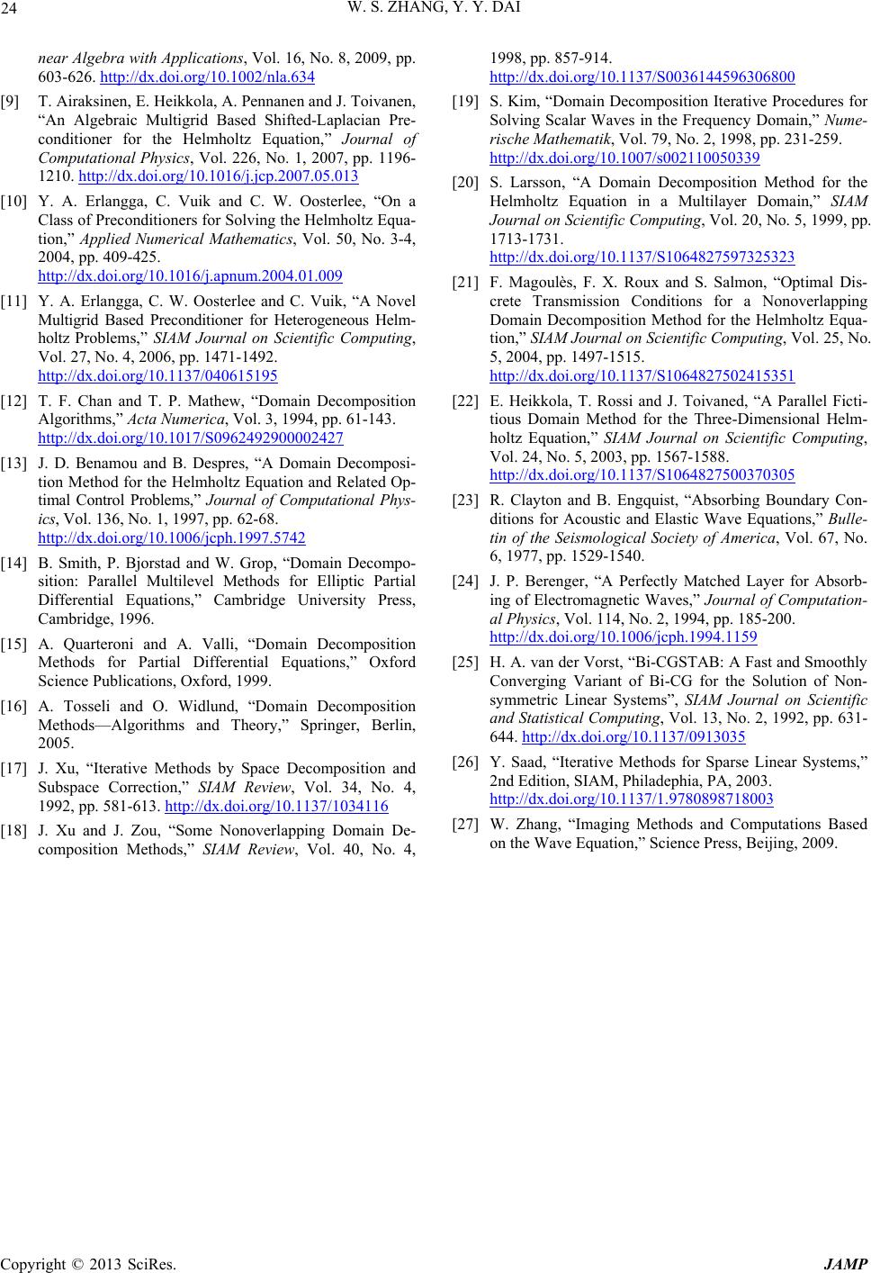

W. S. ZHANG, Y. Y. DAI
24
near Algebra with Applications, Vol. 16, No. 8, 2009, pp.
603-626. http://dx.doi.org/10.1002/nla.634
[9] T. Airaksinen, E. Heikkola, A. Pennanen and J. Toivanen,
“An Algebraic Multigrid Based Shifted-Laplacian Pre-
conditioner for the Helmholtz Equation,” Journal of
Computational Physics, Vol. 226, No. 1, 2007, pp. 1196-
1210. http://dx.doi.org/10.1016/j.jcp.2007.05.013
[10] Y. A. Erlangga, C. Vuik and C. W. Oosterlee, “On a
Class of Preconditioners for Solving the Helmholtz Equa-
tion,” Applied Numerical Mathematics, Vol. 50, No. 3-4,
2004, pp. 409-425.
http://dx.doi.org/10.1016/j.apnum.2004.01.009
[11] Y. A. Erlangga, C. W. Oosterlee and C. Vuik, “A Novel
Multigrid Based Preconditioner for Heterogeneous Helm-
holtz Problems,” SIAM Journal on Scientific Computing,
Vol. 27, No. 4, 2006, pp. 1471-1492.
http://dx.doi.org/10.1137/040615195
[12] T. F. Chan and T. P. Mathew, “Domain Decomposition
Algorithms,” Acta Numerica, Vol. 3, 1994, pp. 61-143.
http://dx.doi.org/10.1017/S0962492900002427
[13] J. D. Benamou and B. Despres, “A Domain Decomposi-
tion Method for the Helmholtz Equation and Relate d Op-
timal Control Problems,” Journal of Computational Phys-
ics, Vol. 136, No. 1, 1997, pp. 62-68.
http://dx.doi.org/10.1006/jcph.1997.5742
[14] B. Smith, P. Bjorstad and W. Grop, “Domain Decompo-
sition: Parallel Multilevel Methods for Elliptic Partial
Differential Equations,” Cambridge University Press,
Cambridge, 1996.
[15] A. Quarteroni and A. Valli, “Domain Decomposition
Methods for Partial Differential Equations,” Oxford
Science Publications, Oxford, 1999.
[16] A. Tosseli and O. Widlund, “Domain Decomposition
Methods—Algorithms and Theory,” Springer, Berlin,
2005.
[17] J. Xu, “Iterative Methods by Space Decomposition and
Subspace Correction,” SIAM Review, Vol. 34, No. 4,
1992, pp. 581-613. http://dx.doi.org/10.1137/1034116
[18] J. Xu and J. Zou, “Some Nonoverlapping Domain De-
composition Methods,” SIAM Review, Vol. 40, No. 4,
1998, pp. 857-914.
http://dx.doi.org/10.1137/S0036144596306800
[19] S. Kim, “Doma in Decomposition Iterative Procedures for
Solving Scalar Waves in the Frequency Domain,” Nume-
rische Mathematik, Vol. 79, No. 2, 1998, pp. 231-259.
http://dx.doi.org/10.1007/s002110050339
[20] S. Larsson, “A Domain Decomposition Method for the
Helmholtz Equation in a Multilayer Domain,” SIAM
Journal on Scientific Computing, Vol. 20, No. 5, 1999, pp.
1713-1731.
http://dx.doi.org/10.1137/S1064827597325323
[21] F. Magoulès, F. X. Roux and S. Salmon, “Optimal Dis-
crete Transmission Conditions for a Nonoverlapping
Domain Decomposition Method for the Helmholtz Equa-
tion,” SIAM Journal on Scientific Computing, Vol. 25, N o.
5, 2004, pp. 1497-1515.
http://dx.doi.org/10.1137/S1064827502415351
[22] E. Heikkola, T. Rossi and J. Toivaned, “A Parallel Ficti-
tious Domain Method for the Three-Dimensional Helm-
holtz Equation,” SIAM Journal on Scientific Computing,
Vol. 24, No. 5, 2003, pp. 1567-1588.
http://dx.doi.org/10.1137/S1064827500370305
[23] R. Clayton and B. Engquist, “Absorbing Boundary Con-
ditions for Acoustic and Elastic Wave Equations,” Bulle-
tin of the Seismological Society of America, Vol. 67, No.
6, 1977, pp. 1529-1540.
[24] J. P. Berenger, “A Perfectly Matched Layer for Absorb-
ing of Electromagnetic Waves,” Journal of Computation-
al Physics, Vol. 114, No. 2, 1994, pp. 185-200.
http://dx.doi.org/10.1006/jcph.1994.1159
[25] H. A. van der Vorst, “Bi-CGSTAB: A Fast and Smoothly
Converging Variant of Bi-CG for the Solution of Non-
symmetric Linear Systems”, SIAM Journal on Scientific
and Statistical Computing, Vol. 13, No. 2, 1992, pp. 631-
644. http://dx.doi.org/10.1137/0913035
[26] Y. Saad, “Iterative Methods for Sparse Linear Systems,”
2nd Edition, SIAM, Philadephia, PA, 2003.
http://dx.doi.org/10.1137/1.9780898718003
[27] W. Zhang, “Imaging Methods and Computations Based
on the Wave Equation,” Science Press, Beijing, 2009.