Journal of Software Engineering and Applications
Vol.12 No.12(2019), Article ID:97364,22 pages
10.4236/jsea.2019.1212033
Optimal Operation Strategies for a Large Multi-Chiller System Based on Cooling Load Forecast
Yanyue Lu1*, Junghui Chen2, Yuanbin Mo1
1School of Chemistry and Chemical Engineering of Guangxi University for Nationalities, Guangxi Key Laboratory for Polysaccharide Materials and Modifications, Key Laboratory of Chemical and Biological Transformation Process of Guangxi Higher Education Institutes, Nanning, China
2Department of Chemical Engineering, Chung-Yuan Christian University, Taiwan

Copyright © 2019 by author(s) and Scientific Research Publishing Inc.
This work is licensed under the Creative Commons Attribution International License (CC BY 4.0).
http://creativecommons.org/licenses/by/4.0/


Received: November 12, 2019; Accepted: November 22, 2019; Published: November 25, 2019
ABSTRACT
In semiconductor and electronics factories, large multi-chiller systems are needed to satisfy strict cooling load requirements. In order to save energy, it is worthwhile to design the chilled water system operation. In this paper, an optimal flexible operation scheme is developed based on a two-dimensional time-series model to forecast the cooling load of multi-chiller systems with chiller units of different cooling capacities running in parallel. The optimal integrity scheme can be obtained using the Mixed Integer Nonlinear Programming method, which minimizes the energy consumption of the system within a future time period. In order to better adapt the change of cooling load, the operation strategy of regulating the chilled water flowrates is employed. The chilled water flowrates are set as a design variable. When the chillers are running, their chilled water flowrates can vary within limits, whereas the flowrates are zero when the chillers are unloaded. This forecasting method provides integral optimization within a future time period and offers the operating reference for operators. The power and advantages of the proposed method are presented using an industrial case to help readers delve into this matter.
Keywords:
Large Multi-Chiller System, Operation Strategies, Cooling Load Forecast, Energy Saving, Optimal Design

1. Introduction
In the high-tech manufacturing industry, such as semiconductor factories and electronics factories, the cooling load is heavy as the plant is strict with the cleanliness and the temperature of air. The power consumption of the chilled water system accounts for about 60% - 70% of the utility cost involved in the high-tech industry [1] [2] [3] [4]. Therefore, it is worthwhile to optimize operation for such a large system since it has tremendous potential in respect of increasing energy efficiency and reducing operating costs.
In order to reduce the energy consumption and make the system in a state of maximum power utilization, commonly an appropriate operating and control scheme is employed. The thermodynamic model of the chiller is the basis for establishing such an operating and control scheme, and a great deal of studies have been made in this aspect. Gordon et al. [5] [6] developed a simple thermodynamic model for the chiller performance using the measured performance data. The model succeeded in predicting the fundamental relation between coefficient of performance (COP) and the cooling rate for the centrifugal chiller. They subsequently expanded the thermodynamic model to explicitly account for the influence of the condenser coolant flow rate and to validate model predictions. Yao et al. [7] investigated a cooling system of residential buildings, and an empirical chiller model was established based on the numerous experimental data. The studies aforementioned are useful to those who want to comprehend the process and to improve the chiller performance. Based on those studies of the chiller unit model, a large number of methods have been developed to design the optimal operating and control scheme for a chiller unit or a chilled water system.
For a single chiller unit, many optimal operation strategies and methods have been developed. Chang [8] used the Lagrangian method to solve the optimal chiller loading problem and to improve the deficiencies of conventional (equal loading rate) methods. Braun et al. [9] [10] developed optimal and near-optimal control strategies using quadratic relationships for chiller systems. In the system-based methodology, an overall empirical cost function of the total power consumption of a chiller plant was developed using a quadratic function. The studies mentioned above focused on improving the chiller’s performance and efficiency by means of experiments and model simulation, and developing a number of theoretical models, empirical models, and semi-empirical chiller models. Most of the models could exactly describe the chiller performance and help to optimize the chiller operation. However, from the viewpoint of energy saving for the whole chilled water system, the interaction between chillers, cooling towers and pumps should also be considered.
For a chilled water system, the efficient operation of the individual unit as well as the whole chilled water system has been studied in some published work. Chan et al. [10] presented a model for designing chiller plants that improves the energy efficiency of the plant in a cost-effective approach. Their design considers the life cycle of the plant and real-time continuous monitoring for better energy management. Surapong et al. [11] explored improving air-conditioning and saving electricity in the spinning industry. They develop a workable control system for the chilled water supply to control the temperature. The results show the potential for saving electricity. Lu et al. [2] [12] presented the global optimization technology for overall heating, ventilating and air conditioning (HVAC) systems. In their research, the characteristics of the major components were introduced by models, and the interactions between them were analyzed and discussed to show the complications of the problem. The global optimization problem was simplified into a compact form and solved using a modified genetic algorithm. Yu and Chan [13] investigated the energy performance of the chiller and the cooling tower systems integrated with the condenser water flow, the speed of cooling tower fans, and the condenser water pumps. Load-based speed control was introduced for the cooling tower fans and the condenser water pumps to achieve the optimum system performance. Most of the control strategies and operation methods mentioned above were applied to public buildings. They were appropriate to the chiller systems that consist of 2 - 4 chillers. Their chilled water system scale is smaller than those of hi-tech factories. Furthermore, the control schedules are obtained based on a point of time in the past research. When the cooling load changes with time, the procedure has to be timely responsive to obtain a new operation scheme.
In this paper, an optimal flexible operation scheme is developed based on a two-dimensional time-series model to forecast the cooling load of multi-chiller systems with chiller units of different cooling capacities running in parallel. The development of the method is very valuable for a large multi-chiller system to save energy. Based on the existing unit model, a system model and its corresponding operating strategy are given. The system model considers the interaction between each unit in a chilled water system by choosing the key control variables, and the matching operating strategy of the large chiller and the small chiller enables the system to adapt the change of the cooling load. Through the novel model expression and the cooling load forecast model, automatic operation of a large chilled water system can be achieved.
2. Problem Description
In high-tech industries, a large set of chilled water systems usually consists of more than 10 chillers with different cooling capacities and several cooling towers (shown in Figure 1). The interactions between different unit operations are complex. Obtaining a proper operation mode of chiller units is not an easy task because the chiller’s performance is affected by several factors, such as the chilled water supply temperature, the partial load ratio and the temperatures of the water entering condenser, etc. In addition, from the viewpoint of energy saving, for the operation of a large set of chilled water systems the load requirement should be considered for the whole period of time instead of a single time point only. In order to obtain an optimal operation scheme of the large set of chilled water systems and to keep the system operation stable without the frequent turning on/off of chiller, an MINLP (Mixed Integer Nonlinear Programming) optimization design method based on the whole period of the cooling load is presented in this paper. Considering the cooling load demand changes

Figure 1. Schematic diagram of a large set of chilled water systems.
with the time, this design method firstly employs a cooling load forecast technique to predict the cooling load of each sub-period within a whole period. Then the operation design problem of the chilled water system can be formulated as the MINLP problem with these predicted cooling loads as constraints, and the design objective is to minimize the system energy consumption in a whole period. In this paper, the MINLP problem can be solved by the mathematical programming method based on the correct expression of the mathematical model and the appropriate choice of the decision variables. Certainly, there are also other approaches that can solve the optimization problem, such as the evolution algorithm; however, it is not the focus of this paper. An integral operation scheme which considers the interaction of different system components and the required cooling loads at different sub-periods can be obtained by solving this MINLP problem. The value of the operation variables, such as the status of chiller loading or unloading, the chilled water flowrate, the cooling water flowrate and temperature, the air flowrate of cooling tower, etc., can be determined simultaneously.
3. Chilled Water System Models
The mathematical programming is adopted to design the system operation scheme, so the system model should be established first. The integrated chilled water system shown in Figure 1 consists of several sets of single chilled water system. It is assumed that a chiller is matched with the corresponding pumps and a cooling tower, and they make up a single chilled water system shown in Figure 2. Since the energy consumption of the chilled water system mainly depends

Figure 2. Schematic diagram of a single chilled water system.
on four primary units, including chillers, cooling towers, chilled water pumps and condenser water pumps, appropriate unit models are required to exactly describe the heat transfer process. The single chilled water system model will be built up based on the empirical and the semi-empirical unit models, in which the interaction among chillers, cooling towers and pumps will be considered.
3.1. Chiller Unit Models
The chiller is a main component of the chilled water system. Its performance affects the system efficiency. The chiller COP is commonly used to evaluate the chiller working efficiency [7] and it is defined as follows:
(1)
where is the power consumption of the chiller. is the quantity of heat transferred to the evaporator. It is equivalent to the chiller’s actual cooling capacity. The evaporator heat transfer (i.e. cooling capacity), , and the condenser heat transfer, , can be calculated based on the energy balance:
(2)
(3)
(4)
where
and
are mass flowrates of the chilled water and the cooling water, respectively.
and
are temperatures of the returning chilled water and the chilled water supply, respectively.
and
are temperatures of the water entering and leaving the condenser respectively.
In the past, many papers have deduced various forms for COP expression. Most of them indicate that COP is related to the partial load ratio (PLR), the evaporator temperature ( ) and the condenser temperature ( ). COP based on [7] is used here,
(5)
(6)
The coefficients, p, q and R, employed in Equation (5) can be estimated by the regression of the operation data. and denote the chiller’s actual cooling capacity and the rated cooling capacity, respectively.
3.2. Cooling Tower Unit Model
Cooling tower is another important unit in chilled water system. The water leaving condenser can be cooled in the cooling tower through processing the heat transfer and the mass transfer between water and air. The states of water and air entering and leaving the cooling tower are important because they simultaneously affect the efficiency of the chiller and the cooling tower. Therefore, an effective model given by Braun [14] that considers the influence is employed here:
(7)
(8)
where is the mass flowrate of the air entering the cooling tower. and denote enthalpies of the air entering and leaving the cooling tower, whereas and denote temperatures of the water entering and leaving cooling tower, and denote respectively moisture contents of the air entering and leaving the cooling tower. and are the mass flowrates of water entering and leaving the cooling tower respectively. Equation (7) & Equation (8) represent the relationships of the energy balance and the mass balance between the cooling water and the air. The heat-rejection capacity of the cooling tower can be calculated by the following equations:
(9)
(10)
where is the heat transfer effectiveness of the cooling tower, and it represents the ratio of the actual enthalpy difference in the air side to the maximum enthalpy difference. of the cross-flow cooling tower is calculated by Equations (11)-(13)
(11)
(12)
(13)
where is the fictitious specific heat defined as the ratio of the enthalpy difference to the temperature difference of the saturation air corresponding to the water entering and leaving the cooling tower. denotes the number of transfer units for measuring the cooling tower performance. It is given by following equations:
(14)
(15)
The coefficients A and p in Equation (14) could be determined based on the measured data under different flowrates of the air and the water. The relationship of physical properties of the moist air employed in the above cooling tower model could be gotten in Refs. [13] [15].
Subsequently, the flowrate of water leaving the cooling tower and the rate of the water loss could be evaluated through the expression of the moisture content and the expression of mass balance [13]. The temperature of the water leaving cooling tower, , is given by Equation (16),
(16)
The required can be satisfied through varying the air flowrate; therefore, a variable-speed fan is required to regulate the air flowrate in the cooling tower. According to the fan law, there is a cubic relationship between the fan power and the flowrate factor,
(17)
3.3. Pump Unit Models
As shown in Figure 1, the chilled water side and cooling water side both need the pumps to transport the circulating fluid. Therefore, the pumps are the main energy consumption unit next to the chiller, which account for over 30% [7]. The refrigerating output of system could be regulated by varying the chilled water flowrate within pump. The energy consumption of pump is related to the flowrate and pumping head; its power is represented by
(18)
where is the weight of water of the unit volume, is pumping head of pump, m is the flow rate, and denotes the efficiency of the pump.
4. Cooling Load Forecasting for a Time Period
Cooling load forecasting is necessary for optimizing operation within a future time period and offering the operating reference for operators. The dynamic design method within a whole period is seldom applied to the operation design of chilled water systems. Most existing design methods are the point-by-point approach, and they can just satisfy the cooling load demand at one time point. When the cooling load is changed, the operation scheme has to be redesigned. The cooling load is adjusted without considering the running chillers at the adjacent time points. This may cause the stability problem of the chiller operation system. The dynamic design method based on the cooling load forecasting can schedule the optimal operation in a whole period and achieve the most economical energy saving. There are various approaches applied to the load forecasting, including multiple linear regression techniques, time-series approaches, artificial neural networks, etc. [16] [17] [18]. Among these methods, the time-series approach is a very attractive forecasting tool because of its simplicity, recursiveness, and economy of use.
Dynamics is an important inherent characteristic of daily operation processes. In some cases, such dynamics exist not only within a particular day but also from day to day. Several different reasons may cause daily-wise dynamics, such as slow property change of refrigerant, drifts of the process characteristics, the effects of slow response variables [17], and so on. All of these reasons are common in daily operation processes. Thus, the dynamics can be viewed with two different time axes: a within-day time axis and a cross-daily time axis, shown graphically in Figure 3. Based on such an idea, a two-dimensional time-series approach is proposed with the within-day time direction as one dimension, and the daily direction as the second dimension. As illustrated in Figure 3, the cooling load data generated by D number of successive days and K sampling intervals of each day are considered. Let
be the cooling load at the sampling interval k in day d (
;
), which can be arranged in a 2-D field with two directions d and k standing for day and time, respectively. This means that the current values of the cooling load
will depend on the past values of the current day in the time direction, 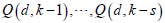 , in day direction,
, and in the cross direction,
, in day direction,
, and in the cross direction,

Figure 3. Two-dimensional representation of the cooling load data.
, where and s are the autoregressive orders in the two directions. The region covering the lagged values above is shown in Figure 3. Mathematically, the forecasting model is expressed as:
(19)
where a, b and c are the regression coefficients. The above equation is similar to the conventional time series identification, but it includes the within-day time direction as one dimension as well as has the daily direction as the second dimension,
5. Optimal Operation Design Model Formulation
When the cooling load changes, it would be preferable to adjust the operation scheme according to the requirement of cooling capacity. Therefore after the cooling load at each sub-period point is predicted, the design method presented in this paper would give an operation scheme within the future time period. This design scheme can offer an operating schedule for operators to enhance the performance of the chilled water system and to keep the system operation stable.
In addition, for a large chilled water system in the hi-tech industry, the chillers are the main source of energy consumption. The frequent operation of turning on/off chillers may save energy to a certain degree when the cooling load is changed, but it is not conducive to maintaining the system stability and extending the chillers’ life span. Instead of the system design at a point of time, the operation scheme obtained from the optimization design within a time period can prevent the disadvantages mentioned above, as the interaction of chiller running state between sub-time periods is considered. The objective of this design is to minimize the operation cost J in the whole time period, which can be described by Equation (20).
(20)
s.t. (21)
(22)
(23)
(24)
where the subscript i denotes sub-time period i. The length of the period is I. For the design of operation stability, two sizes of the chillers are classified, where N and M denote the number of large-sized chillers and small-sized chillers, respectively. denotes the power consumption of the nth large chiller at the ith time point. , and denote the power consumption of the chilled water pump, the condenser water pump and the cooling tower fan, respectively, and they are equipped with the large chillers. Analogously, ,,, and denote the corresponding power consumption of the small chillers. is a binary variable; when it is 1, the chiller is running during the ith sub-period; on the other hand, when it is 0, the chiller is turned off. is the energy charge. and denote the costs of the large and the small chillers from the beginning till reaching a steady operation.
In order to maintain the system’s stability and avoid frequent loading or unloading of the chillers, the fixed cost of the chiller starting up should be calculated when the chillers are loaded. The first term of the right side in Equation (20) is used to determine when the fixed cost of the large chiller loading should be calculated. is a binary variable and its value is determined by constraints Equation (21) and Equation (22). Analogously, the operating logics for the starting up cost of the small chiller could be guaranteed by the constraints of Equation (23) and Equation (24), where U is a large positive integer.
Besides the fixed cost of the chiller loading, the system operation cost depends on the energy consumption of chiller, cooling tower and pump. Their power consumption in Equation (20) can be calculated by the unit models presented above. In this paper, the operation strategy of regulating the chilled water flowrates is employed. The chilled water supply temperature and chilled water returning temperature are fixed values, while the chilled water flowrates are design variables. When the chillers are running, its chilled water flowrate can vary within limits, whereas the flowrate is zero when the chillers unload. The relationship between chiller running status and the value of chilled water flowrate can be defined by following logical constraints:
(25)
(26)
In Equation (25), and are the low bound and up bound of chilled water flowrate of nth large chiller, respectively. is the chilled water flowrate of nth large chiller within the ith sub-time period. Analogously, Equation (26) is the logical constraint about small chillers. According to mass balance and energy balance, the chilled water flowrate relates to the power consumption of chiller, cooling tower fan and pump. In this way, the refrigerating output of system could be regulated by the chilled water flowrate to adapt to the cooling load requirement change. Following constraints guarantee the sufficient refrigerating output to satisfy the demand of air-conditioning:
(27)
(28)
where indicates the total chilled water flowrate of system. is the system cooling load at ith time point, its value is equal to the predicted cooling load Q in Equation (19). According to above mathematical models, the optimal operation can be designed by expressing the problem as a mixed integer nonlinear programming in which the objective function is Equation (20), designed variables include the chilled water flowrates ( ), the partial load ratio (PLR), the water temperatures entering the condenser ( ), the cooling water flowrates ( ), the air flowrate entering the cooling tower ( ), and all the binary variables.
The design method proposed above is an approach based on the prediction of cooling load. The design results would yield an operating scheme of the chilled water system which can provide a reference for operators. If the measured practical cooling load is different from that of the predicted one, the predicting model of the cooling load will be updated by the latest collected data. Consequently, the new operating design of the chilled water system will be close to the practical requirement of the cooling load. These updated operations are easily realizable since all steps are programmed. To illustrate the proposed design method, the operating scheme of chilled water system in a working day will be discussed in the following case study.
6. Case Study
For the purpose of illustrating the effectiveness of the proposed methodology, three cases are discussed. The first two cases use different operating modes for the same chilled water system consisting of large-sized chillers and small-sized chillers. The third case simulates the real plant which consists of only large-sized chillers, and uses the operating mode of average load. Most of the data employed in these cases come from the chilled water system of a semiconductor factory in Taiwan. The design method presented in this paper is effective in saving the potential operating cost in this factory.
For the first two cases, it is assumed that the chilled water system consists of 8 large chillers (1750 RT) and 2 small chillers (500 RT). Each chiller is equipped with a chilled water pump, a condenser water pump and a cooling tower. Table 1 and Table 2 summarize the detail of chilled water systems with the large and the small chillers. Case 1 employs the operating mode of changing load that is proposed in this paper, the load of each chiller can change with the external cooling load by regulating the output flowrate of chilled water. On the other hand, Case 2 uses the operating mode of average load, which is the common operating method.
In order to determine the parameters of these chiller unit models, a great deal of operational data are collected. The empirical relationship of the chiller’s COP shown in Equation (5) is used to evaluate the chiller efficiency. The parameters in Equation (5) for the large chillers are listed as follows:
(29)
For the small chillers, the regressed parameters in Equation (5) are listed below:
(30)

Table 1. Detail of the chilled water system with the large chillers.
Table 2. Detail of the chilled water system with the small chillers.
PLR is a key variable in Equation (5). The value of COP is more sensitive to the change of PLR. In general, for the sake of the energy saving, the chillers are operated within a certain range of PLR which can maximize COP. For this chilled water system of the semiconductor factory, when the evaporator temperature ( ) and the condenser temperature ( ) are fixed at 9˚C and 32˚C, the relationships of the large chillers and the small chillers between COP and PLR are given in Figure 4 and Figure 5, respectively. From the two figures, it is found that the values of COP are relatively high within the PLR scope of 0.7 - 0.8 for these two types of chillers. In this PLR scope, the chillers would obtain high operation efficiency.
Before executing the optimal operation design of this chilled water system, predicting the cooling load of the whole duration is essential. In this case study, the cooling load data from April 8 to 20 are collected to predict the cooling load on April 21 using the aforementioned two-dimensional time-series approach. The forecasted results of the cooling load during 8:00a.m. - 6:00p.m. on April 21 are plotted in Figure 6. In Figure 6, the blue points represent the actual load at each time point; the black line is the forecasted cooling load. For the short-term load forecasting, the two-dimensional time-series approach can make an effective prediction. Then the MINLP optimization problem based on the forecasting cooling load can be solved using the GAMS/DICOPT software to minimize the operation cost within the design period.
Owing to the computation hardness of MINLP problem, in this case, the whole time period showed in Figure 6 was divided into 6 sub-time periods by 5
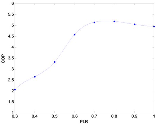
Figure 4. Relationship of COP and PLR of the large chillers.
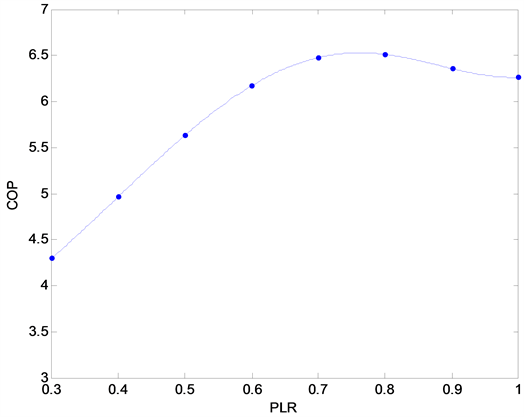
Figure 5. Relationship of COP and PLR of the small chillers.
time points, i.e. 9, 11, 13, 15, 17 o’clock. The system operation scheme within the whole time period would be designed with these predicted cooling loads of 5 time points as constraints. The refrigerating output at these time points must meet the cooling load. For MINLP problem, several initial values were tried to obtain a solution that is close to the global optimum. The design results for the three cases are presented in Tables 3-5, respectively.
Figure 6. Results of the cooling load prediction.
(a) (b)
Table 3. Design results of the operation scheme for the chilled water system in Case 1.
6.1. Operating Mode of Changing Load
Case 1 uses the operating mode of changing load to regulate the chilled water flowrate of each chiller. The mathematical model of this case includes all the equations in Section 3. The design results of this case are listed in Table 3. Its total
(a) (b)
Table 4. Design results of the operation scheme for the chilled water system in Case 2.
Table 5. Design results of the operation scheme for the chilled water system in Case 3.
system cost within the whole duration is $8220.4. From Table 3, it can be seen that the chillers are all loaded within the whole period, but the refrigerating output of some chillers are different when the cooling load change. The chiller efficiency analysis has proved that when the value of PLR is within 0.7 - 0.8, the chiller efficiency for these two sizes is maximized. Therefore when the cooling load is relatively small, some chiller’s PLR are kept close to this range to ensure a relatively high efficiency of the overall system. With increased cooling load, most chillers have to run under full load status. By using the variable load of the distribution method and regulating chilled water flowrate, a better system performance of the chilled water system is obtained. From the design results, it can also be seen that it is beneficial to run both large chillers and small chillers together. The small-sized chillers are used for the minor adjustment with regard to the small difference in the required load based on the current operation capacity. In this way, the system would remain stable.
6.2. Operating Mode of Average Load
Case 2 uses the operating mode of average load. In this case, the flowrates of chilled water in the system are also set to be variables, but the flowrates are unified for the same type of chiller. Besides all the equations presented in Section 3, the mathematical model of this case includes the constraints of equal chilled water flowrates. The design results of this case are listed in Table 4. The total system cost within the whole duration is $8356.6. Table 4 shows that the small-sized chillers are not used during the early stage while all the large-sized chillers are running with big load. With the increase of cooling load, the small-sized chillers are loaded, and they are unloaded gradually with the decrease of cooling load. As the same type of chillers takes on the same cooling load which changes with time, all the chillers have to be frequently regulated when the time changes from one sub-time period to another in this case. Whereas, the number of chillers in Case 2 which need to be regulated within different sub-time periods is greater than those in Case 1, if the relevant control equipment is limited, the operating mode used in Case 2 may be easier for operation since the change of flowrate is unified. In practice, the timing of using which one of these two operating modes depends on the site conditions. From the viewpoint of energy saving, the system power consumption in this case is more than that of Case 1 because the former provides excessive cooling capacity.
6.3. Large-Sized Chillers System
For comparison, Case 3 simulates the real plant which consists of nine large-sized chillers, and uses the operating mode of average load. The parameters of this chilled water system are presented in Table 1. Its mathematical model is the same as the one in Case 2, excluding the unit model of the small-sized chiller. The design results of this case are listed in Table 5 which was validated by comparing with process data coming from real plant. It is found that the chilled water flowrate of all the chillers has to be frequently regulated within the whole duration to satisfy the cooling load requirement of different sub-time periods. The total system cost within the whole duration is $
The cost comparisons in Table 6 show that Case 1 has the least total cost
Table 6. The cost comparison of three cases.
among the three cases due to the less power consumption. For the same chilled water system, the system using the operating mode of changing load consumes less power than that using the operating mode of average load. For different chilled water systems, the system consisting of two sizes of chillers has less fixed and operating costs than that of only large-sized chillers since the former can provide a more flexible and stable operation.
7. Conclusions
An MINLP method has been presented for the operation design of a large multi-chiller system, which could provide an integral operation scheme within a whole period based on the cooling load forecast. For accurate prediction of the cooling load, a two-dimensional time-series approach is presented with the within-day time direction as one dimension and the daily direction as the second dimension. Some conclusions can be drawn as follow:
1) Instead of the general method at one time point only, this forecasting scheme can offer an operating reference for operators to enhance the energy performance of the chilled water system and to keep the system operation stable.
2) The operation design problem during a whole time period is formulated as an MINLP problem. It is an integral operation scheme since it considers the interaction of different system components and different sub-period which results in better energy saving.
3) Three cases study illustrate the significance of this design method. The design results indicate that the collocation running mode of the large chillers and the small chillers can efficiently reduce the chiller system energy consumption through properly adjusting the refrigerated output when the cooling load varies.
The strategy in this paper focuses on the theoretical development of the design methodology and the mathematical expression of models; it is not developed for specific cases at this stage. However, it can provide a universal reference for the design of the operating scheme of large chilled water systems. The unit models involved in this design method can be changed or substituted by other appropriate unit models according to actual requirements on site. They do not affect the performance of the design method. The feasibility and validity of this method have been approved in the simulation cases, i.e. Case 2 and Case 3, which display the common operating situation in real plants.
Acknowledgements
The authors wish to express their sincere gratitude to the National Science Council, R.O.C., the National Natural Science Foundation of China (No.21566007), (No.21968008) and (No.21466008), and the Guangxi Natural Science Foundation (2018GXNSFAA050025) for their financial support.
Conflicts of Interest
The authors declare no conflicts of interest regarding the publication of this paper.
Cite this paper
Lu, Y.Y., Chen, J.H. and Mo, Y.B. (2019) Optimal Operation Strategies for a Large Multi-Chiller System Based on Cooling Load Forecast. Journal of Software Engineering and Applications, 12, 540-561. https://doi.org/10.4236/jsea.2019.1212033
References
- 1. Hodge, B.K. and Taylor, R.P. (1999) Analysis and Design of Energy Systems. Prentice Hall, Upper Saddle River, NJ.
- 2. Lu, L., Cai, W., Chai, Y. and Xie, L. (2005) Global Optimization for Overall HVAC Systems Part I Problem Formulation and Analysis. Energy Conversion and Management, 46, 999-1014. https://doi.org/10.1016/j.enconman.2004.06.012
- 3. Wang, S.W. and Ma, Z.J. (2008) Supervisory and Optimal Control of Building HVAC Systems: A Review. HVAC & R Research, 14, 3-32. https://doi.org/10.1080/10789669.2008.10390991
- 4. ASHRAE (2007) ASHRAE Handbook—HVAC Applications (SI), Supervisory Control Strategies and Optimization, Chapter 41. American Society of Heating, Refrigerating and Air-Conditioning Engineers Inc., Atlanta, GA.
- 5. Gordon, J.M., Ng, K.C. and Chua, H.T. (1995) Centrifugal Chillers: Thermodynamic Modelling and a Diagnostic Case Study. International Journal of Refrigeration, 18, 253-257. https://doi.org/10.1016/0140-7007(95)96863-2
- 6. Gordon, J.M., Ng, K.C., Chu, H.T. and Lim, C.K. (2000) How Varying Condenser Coolant Flow Rate Affects Chiller Performance: Thermodynamic Modeling and Experimental Confirmation. Applied Thermal Engineering, 20, 1149-1159. https://doi.org/10.1016/S1359-4311(99)00082-4
- 7. Yao, Y., Lian, Z.W. and Hou, Z.J. (2004) Optimal Operation of a Large Cooling System Based on an Empirical Model. Applied Thermal Engineering, 24, 2303-2321. https://doi.org/10.1016/j.applthermaleng.2004.03.006
- 8. Chang, Y.C. (2004) A Novel Energy Conservation Method—Optimal Chiller Loading. Electric Power Systems Research, 69, 221-226. https://doi.org/10.1016/j.epsr.2003.10.012
- 9. Braun, J.E. and Diderrich, G.T. (1990) Near-Optimal Control of Cooling Towers for Chilled-Water Systems. ASHRAE Transactions, 96, 806-813.
- 10. Chan, K.L., Lee, W.M. and Yuen, K.K. (2011) An Integrated Model for the Design of Air-Cooled Chiller Plants for Commercial Buildings. Building and Environment, 46, 196-209. https://doi.org/10.1016/j.buildenv.2010.07.013
- 11. Surapong, C., Liu, B., Nguyen, H.Q. and Tian, W. (1996) Improving Air-Conditioning and Saving Electricity in the Spinning Industry. Energy Sources, 18, 627-635. https://doi.org/10.1080/00908319608908795
- 12. Lu, L., Cai, W., Chai, Y. and Xie, L. (2005) Global Optimization for Overall HVAC systems—Part II Problem Solution and Simulations. Energy Conversion and Management, 46, 1015-1028.
- 13. Yu, F.W. and Chan, K.T. (2008) Optimization of Water-Cooled Chiller System with Load-Based Speed Control. Applied Energy, 85, 931-950. https://doi.org/10.1016/j.apenergy.2008.02.008
- 14. Braun, J.E. (1988) Methodologies for the Design and Control of Chilled Water Systems. Ph.D. Thesis, University of Wisconsin-Madison, Madison, WI.
- 15. Ponce-Ortega, J.M., Serna-González, M. and Jiménez-Gutiérrez, A. (2007) MINLP Synthesis of Optimal Cooling Networks. Chemical Engineering Science, 62, 5728-5735. https://doi.org/10.1016/j.ces.2007.05.014
- 16. Soliman, S.A., Persaud, S. and El-Nager, K. (1997) Application of Least Absolute Value Parameter Estimation Based on Linear Programming to Short-Term Load Forecasting. International Journal of Electrical Power & Energy Systems, 19, 209-216. https://doi.org/10.1016/S0142-0615(96)00048-8
- 17. Yao, Y., Lian, Z.W., Liu, S.Q. and Hou, Z.J. (2004) Hourly Cooling Load Prediction by a Combined Forecasting Model. International Journal of Thermal Sciences, 43, 1107-1118. https://doi.org/10.1016/j.ijthermalsci.2004.02.009
- 18. Hahn, H., Meyer-Nieberg, S. and Pickl, S. (2009) Electric Load Forecasting Methods: Tools for Decision Making. European Journal of Operational Research, 199, 902-907. https://doi.org/10.1016/j.ejor.2009.01.062
Symbols
: enthalpy of air entering the cooling tower (kJ/kg)
: enthalpy of air leaving the cooling tower (kJ/kg)
: enthalpy of saturation air corresponding to the temperature of water entering the cooling tower (kJ/kg)
: enthalpy of saturation air corresponding to the temperature of water leaving the cooling tower (kJ/kg)
COP: coefficient of performance of the chiller
: state variable
: specific heat capacity of water (kJ/(kg˚C))
: evaporator state variable
: condenser state variable
N: number of transfer units of the cooling tower
: mass flowrate of air entering the cooling tower (kg/s)
: rated flowrate of air entering the cooling tower (kg/s)
: mass flowrate of chilled water (kg/s)
: mass flowrate of water entering the condenser (kg/s)
: mass flowrate of water entering the cooling tower (kg/s)
: mass flowrate of water leaving the cooling tower (kg/s)
: state variable
: power consumption of the chiller (kW)
: power consumption of the cooling tower fan (kW)
: rated power consumption of the cooling tower fan (kW)
: power consumption of the pump (kW)
PLR: partial load ratio of the chiller
: heat transfer quantity of the evaporator (equivalent to the chiller cooling capacity) (kW)
: rated cooling capacity (kW)
: heat transfer quantity of the condenser
: evaporating temperature (˚C)
: condensing temperature (˚C)
: chilled water returning temperature (˚C)
: chilled water supply temperature (˚C)
: condenser water entering temperature (˚C)
: condenser water leaving temperature (˚C)
: temperature of water entering the cooling tower (equivalent to ) (˚C)
: temperature of water leaving the cooling tower (equivalent to ) (˚C)
: time interval
Z: binary variable
: moisture content of air entering the cooling tower (kg/kg dry air)
: moisture content of air leaving the cooling tower (kg/kg dry air)
: airside heat transfer effectiveness of the cooling tower
: specific weight of water (kN/m3)
: efficiency of the pump