Journal of Service Science and Management
Vol.10 No.01(2017), Article ID:74333,15 pages
10.4236/jssm.2017.101003
Study on the Dynamic Relationship between Housing Price and Land Price in Shenzhen Based on VAR Model
Zuqiu Wen
School of Business Administration, South China University of Technology, Guangzhou, China
![]()
Copyright © 2017 by author and Scientific Research Publishing Inc.
This work is licensed under the Creative Commons Attribution International License (CC BY 4.0).
http://creativecommons.org/licenses/by/4.0/


Received: January 18, 2017; Accepted: February 21, 2017; Published: February 24, 2017
ABSTRACT
Irrational growth in the real estate market of first-tier cities once again triggered a discussion on the relationship between housing price and land price. This paper uses the quarterly data of housing price and land price of Shenzhen from 2003 to 2015 to establish VAR model which is based on unit root test, co-integration test and analysis of Error Correction Model, and then it makes an empirical study on the relationship between housing price and land price of Shenzhen through analysis frame of impulse response function and variance decomposition. The research shows that there is a long-term equilibrium relationship between housing price and land price in Shenzhen: in the long term, housing price determines land price, while in the short term, they interact with each other; Shenzhen’ housing price and land price are affected by themselves very much, its real estate market’s financial attribute is becoming more and more prominent. Finally, this paper puts forward some corresponding policy recommendations to stabilize the real estate market based on the results of this study.
Keywords:
Housing Price, Land Price, VAR Model, Impulse Response Function, Variance Decomposition

1. Introduction
Since the housing becomes commodity supplied and the land becomes market oriented, national economy developed sustainably, housing system reformed constantly, urbanization process grown up rapidly and real estate developed vigorously. Commercial housing market has gradually been in the dominant position. But since 2015, the first-tier cities appear “land kings” constantly, high premium transaction has become the norm; housing price also continues to increase. In early 2016, the largest increase of new commercial housing price index was in Shenzhen, where rose 52.7% year on year and refresh people’s cognition repeatedly [1] . The continuously rising of housing price not only closely related to people’s livelihood, but also threatened to the economic development and social stability.
What’s the dynamic relationship between housing price and land price which are two important indicators in the real estate market? Whether there is a Granger causality relationship between them? What are the dynamic effects of a change in one variable will have on the system? How great the effect will be? Clarify these issues is of great significance for the scientific formulation of policy and promoting the development of the real estate market healthily.
At present, scholars have made a lot of research on the dynamic relationship between housing price and land price and have achieved some theoretical results. Zhangtonglong studied the relationship between housing price and land price by using quarterly data from 1998 to 2009 through establish vector error correction model, the results show that there is a long-term equilibrium relationship between housing price and land price, and the cause-and-effect relationship is that housing price determines land price [2] . Kuangweida used the national housing price index and land price index from the 1 quarter of 1999 to the 1 quarter of 2005 and established a ECM model to test them, the results show that in the short term housing price and land price are mutually Granger causality, in the long-term land price is the Granger reason of the housing price [3] . Songbo and Gaobo used quarterly data of housing price and land price from 1998-2006 to test the causal relationship through the establishment of vector autoregressive, the result showed that in the short term housing price makes no impact on the land price while the land price is the Granger reason of the housing price, in the long run housing price and land price have the two-way causal relationship [4] . Longhaiming and Guowei established a VAR model to study the relationship between housing price and land price by using the quarterly data of the national housing sales price index and the land transaction price index from 1999-2008, the results showed that there was a long-term interaction mechanism between housing price and land price, the impact of housing price on land price was greater than the impact of land price on housing price [5] . Sunbo thinks the local government over reliance on “land finance” which causes the land price rising greatly and improves a speculative demand for land, finally the expectation of housing price continues to pull the housing price and lead to further increases of land price. In this process, land price and housing price condition each other, and form a price spiral [6] . From the existing literature, there are three main points of view: the first is derived demand view, it considers the land price as a derived demand of the housing price, the increase of land price is the consequence of the increase of housing price instead of the reason [7] [8] ; the second is cost drive view, it thinks that land price makes the largest proportion of the housing price, so housing price is determined by the land price to a large extent [9] [10] ; the third is that housing price and land price influence each other [11] [12] [13] .
Generally speaking, the present research has carried on a series of discussion on the relationship between housing price and land price, however, they haven’t get a accordant conclusion on this problem. If we take carefully look at these studies we will find they have the following deficiencies: 1) In data analysis, some thesis do not take the stability of variables into account, only stationary time series can be used to analyze the causal relationship between variables based on Granger causality test; There are also some thesis whose time series is too short due to the availability of the data which resulting in inconsistent results; And there are also some thesis which choose different variables to make the study [14] [15] . 2) Previous studies used the national conceptual data to analyze the relationship between housing price and land price in China. However, the real estate market is a regional market which has strong local characteristics, there are great differences in economic development, geographic conditions and factor endowments between different cities. Therefore the relationship of housing price and land price is different in different cities and we must consider the individual differences in order to grasp the real situation of the interaction between housing price and land price and come to a practical conclusion [16] [17] .
In summary, in order to solve the problem of data processing in the existing studies and considering the regional differences between different cities, this paper chooses Shenzhen’s real estate market as the research object, and uses the quarterly data of housing sales price index and land transaction price index as a sample from 2003 to 2015 and established the VAR model, which was based on the results of unit root test and co-integration test, and then made an empirical study by using impulse response function (IRF) and variance decomposition (VD). In the end, this paper put forward some corresponding policy recommendations in order to make the real estate market develop steadily and healthily.
2. Data Description and Theoretical Model
2.1. Data Description
In this paper we choose “housing sales price index (HP)” and “land transaction price index (LP)” of Shenzhen as the research variables, The data comes from the “Chinese Statistical Yearbook”, “China Monthly Economic Indicators”, and “China urban land price Dynamic monitor website”. The sample space of this paper is from the first quarter of 2003 to the fourth quarter of 2015 with a total of 52 time series data. We fixed other data based on HP and LP of the first quarter of 2003. In order to eliminate the influence of abnormal data on the estimation accuracy of the model, the variable data are used in the form of logarithm. Take:
LHP = Ln(HP) Natural logarithm of housing price index
LLP = Ln(LP) Natural logarithm of land price index
In this paper, the calculation process is all completed by using Eviews 8.
2.2. Error Correction Model
Econometrics theory points out that we could establish an Error Correction Model to carry out long-term equilibrium test and Granger causality test if the two time series are of the same order and with a co-integration relationship.
The mathematical expression of ECM model is:
 (1)
(1)
 (2)
(2)
Among them,  and
and  are error correction term,
  and
and  are adjustment factor; i and j are Lag length;
  and
and  are perturbation term which obey normal distribution.
2.3. VAR Model
VAR model is a kind of non-structured equation model which takes each of the endogenous variables in the economic system as a function of the lagged values of all endogenous variables. It always used to forecast interconnected time series systems and analysis the dynamic impact of random disturbance on the variable system and then it could explain the impact of various economic shocks on the formation of economic variables.
The mathematical expression of VAR model is:
![]() (3)
(3)
Among them, ![]() is k dimensional endogenous variable column vector,
is k dimensional endogenous variable column vector, ![]() is d dimension exogenous variable column vector, p is lag length, T is the sample number. Matrix
is d dimension exogenous variable column vector, p is lag length, T is the sample number. Matrix![]() , …,
, …, ![]() and matrix H is coefficient matrix which need to be estimated.
and matrix H is coefficient matrix which need to be estimated. ![]() is perturbed column vector with K dimension, they can be related to each other, but it can’t related to its lag value and variables on the right side of the equation.
is perturbed column vector with K dimension, they can be related to each other, but it can’t related to its lag value and variables on the right side of the equation.
2.4. Impulse Response Function
Because the VAR model is a kind of non-theoretical model in application, therefore, in the analysis of VAR model, we often do not analyze the influence of one variable have on another variable, but analysis the case when an error term is changed or when the model is hit by some sort of shock, what the dynamic effects of the system will be, we call this method the Impulse response function method. It can provide information about the positive and negative direction of the response, the adjustment of the time delay and the stabilization process generated by the impact of the system. Combined with the research of this paper, the result of impulse response function can describe the dynamic process of housing price and land price changes caused by a variable change in housing price and land price. In the following we take VAR (2) model as an example to illustrate the basic idea of impulse response function.
![]() (4)
(4)
Among them,![]() ; ai, bi, ci, di are parameters to be estimated,
; ai, bi, ci, di are parameters to be estimated, ![]() = (
= (![]() ,
, ) is perturbation term, and assume that they are white noise vectors with the following properties:
 (5)
(5)
Assume that the system starts from the 0 phase, and set x1 = x2 = y1= y2= 0, the zeroth period is given a perturbation term  = 1,
= 1,  = 0, and the following are all 0, that means
  =
=  = 0 (t = 1, 2,…), Call this “give X a impulse at 0 phase”. The impulse between xt and yt is: when t = 0, x0 = 1, y0 = 0; bring the results to the response function, when t = 1, x1 = a1, y1= c1; and then bring the results into the response function, when t = 2,
  ,
,  . The initial disturbance will be transmitted in the system. It can be obtained by iterative calculation about x0, x1, x2, x3, etc. We call them the X response function caused by the pulse of X. In the same way, we can calculate y0, y1, y2, y3, etc. We call them the Y response function caused by the pulse of X. we can obtain X response function and Y response function caused by the pulse of Y When the zeroth phase of the pulse is
  = 0,
= 0,  = 1.
= 1.
Through the above impulse response process we can clearly capture the dynamic changing process of the housing price and land price caused by the housing price and land price.
2.5. Variance Decomposition
The variance decomposition is through analysis the change of contribution degree of the endogenous variables impacted by each structure, and then gives information about the relative importance of each random disturbance to the variables in the system, which can evaluate the importance of the impact of different structures. Its basic principles are as follows:
 (6)
(6)
Among them, . Each content in parentheses is the impact
  has on yi from the infinite past to the present time. Assume that
  has no sequence correlation:
 (7)
(7)
Assume that the covariance matrix Σ of perturbation vector is the diagonal matrix, so:
Among them, . The variance of yi can be decomposed into k species which not related to each other. In order to determine the extent each disturbance term has on the variance of Y, we define the dimension as follows:

The relative variance contribution rate (RVC) is based on the relative contribution of impact based variance j variable had on variance of yi and then observe the effects of j variable make on  variable.
In fact, it is impossible to use  when the variable is until infinity, if the model satisfies the stationary condition
  shows a geometric progression with the increase of q variable, so we just need to take a limited items of q variable.
3. Empirical Test on the Relationship between Housing Price and Land Price
Based on adjusted housing price index and land price index we drew the time sequence graph as below, from the Figure 1 we can see that both the housing price and land price are all showed an upward trend, the volatility of the housing price index is significantly higher than the housing index and there is a strong correlation between them.
3.1. Stability Test of Variables
According to the relevant theory of econometrics, in the analysis of time series of economic variables, we should first test the stability of the variables, otherwise there will be false regression. If the variable is not a stationary time series, we can make a difference on the variables until the sequence is stable. If the sequence is stable after n times difference, we say the original sequence is a single integer sequence of order n, and denote it a I(n). The method we often used to make stability test are DF test, ADF test, etc. This paper uses the ADF test method, the test results are shown in Table 1.
As can be seen from Table 1, the statistic of sequence LLP and ADF is greater than the critical value of the 5% significant level, so we can’t reject the original hypothesis that the original time series is a non-stationary sequence; while the ADF statistic of ΔLHP and ΔLLP is less than the critical value of 5% significant level, so they are all stationary time series. Therefore, the LHP sequence and LLP sequence are all integrated of order 1.
3.2. Long Term Equilibrium Relationship Test
From the previous analysis, we can know that the sequence of LLP and LHP are all integrated of order 1, they satisfy the conditions of co-integration test, so there may be a co-integration relationship between the two variables. In this paper, we use Johansen test to determine whether there is a co integration relationship between them, and the results are shown in Table 2.
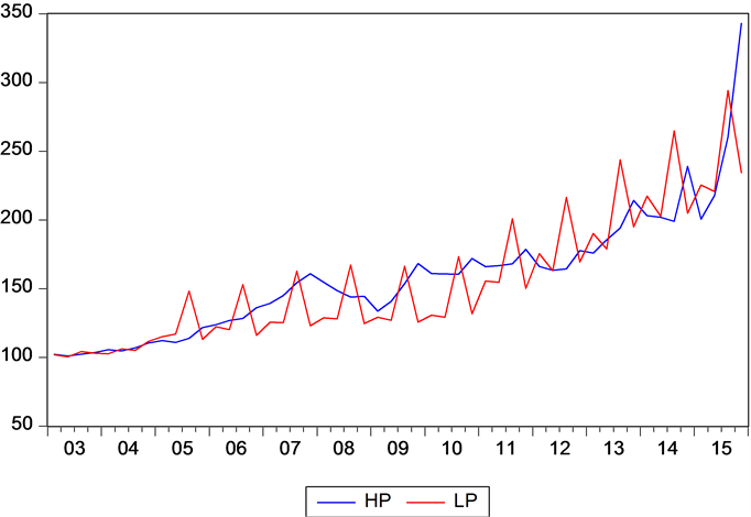
Figure 1. Time sequence diagram of housing price and land price.

Table 1. ADF unit root test results.
Note: Δ represents two order difference; in the testing method, C represents the constant term, T represents the trend term; the lag length is determined by the AIC minimum criterion.
From the test results, when the original hypothesis R = 0, trace statistic value of 18.57133 is greater than the 5% level of the critical value of 12.3209, thus rejecting the null hypothesis; when the original hypothesis , trace statistic value of 3.491727 is below the 5% level of the critical value of 4.129906, thus accept the original hypothesis. This shows that there is a long-term stable co-inte- gration relationship between LHP and LLP.
3.3. Error Correction Model Analysis
After confirming the co-integration relationship between LHP and LLP, we can establish the error correction model to analyze their cause and effect relationship. Table 3 lists the results of the error correction model.
From the test results we can find the following conclusions:
First, in the examination of land price to housing price the error correction item for long-term effects is not significant, while in the examination of housing price to land price the error correction item is significant. This shows that the long-term equilibrium relationship between them is that the housing price affect the land price.
Table 2. Johansen test results.
Table 3. Test results of error correction model.
Note: in the brackets are the corresponding T statistics.
Second, in the short term, the first lag difference of land price to housing price is significant while the others are not; the first lag difference and second lag difference of housing price to land price are all significant. This shows that in the short term, housing price and land price have the cause and effect relationship.
Finally, in the equation of land price to housing price, the first lag difference of housing price is significant, in the equation of housing price to land price, the first lag difference of land price is significant. This shows that the lag of housing
price and land price have explanatory power to the change of themselves. It can be seen that expected factors play a certain role in the formation of their respective prices.
In summary, in the long term, housing price is the Granger reason of land price, land price is not the Granger reason of housing price; in the short term, there exists a Granger cause and effect relationship between housing price and land price.
3.4. Construction and Estimation of VAR Model
Based on stability test and co-integration test, combined with the basic idea of VAR model, we established a VAR model with the time series data of housing price and land price.
According to the AIC and SC information criterion, the optional lag length is 3. We use Eviews 8 to estimate the parameters of VAR model and the result is as follows:
LHP = −0.1454 + 1.178LHP(−1) − 0.4311LHP(−2) + 0.135LHP(−3)
(−0.836) (6.5158) (−1.7515) (0.8522)
+ 0.2874LLP(−1) − 0.2063LLP(−2) + 0.0702LLP(−3)
(4.5241) (−2.766) (0.8068)
LLP = −0.271 − 0.0412LHP(−1) − 0.8665LHP(−2) + 1.3775LHP(−3)
(−0.7184) (−0.1050) (−1.6227) (4.0070)
+ 0.0271LLP(−1) + 0.3849LLP(−2) + 0.1833LLP(−3)
(0.1969) (2.3789) (0.9714)
3.5. Impulse Response Analysis and Variance Decomposition Analysis
In order to analyze the dynamic impact between housing price and land price and the contribution of each structure impact to the change of endogenous variables, this section we use impulse response function and variance decomposition to make further analysis for them.
1) Impulse response analysis
The impulse response results are shown in Figure 2(a) and Figure 2(b), the horizontal axis represents the tracking period of the impulse response function, the vertical axis represents response degree the explanatory variable had on the explained variable. Figure 2(a) reflects the dynamic response of housing price which was shocked by a standard deviation of endogenous variables: LHP immediately had a strong reflection after being hit by a standard deviation shock of its own, its price fluctuation increases 5.4 percent and rises rapidly, and reached the maximum value of 7.2 percent in the second period, then continued to decline, reaching a minimum of 3.3 percent in the fourth period, from the fifth phase it began to rise and remained increase. LHP did not respond in the first period after a standard deviation shock from LLP, in the second period it increased to 3.2 percent, then in the third period it dropped to 1.6 percent, and in the fourth period rose to 2.4 percent, after that it appeared seasonal fluctuation, and the fluctuate began to slow down after eight phase, the overall reflection intensity is lower than its own inertia.
Figure 2(b) reflects the dynamic response of land price which was shocked by a standard deviation of endogenous variables: LLP immediately had a very strong reflection after being hit by a standard deviation shock of its own, its price fluctuation increases 11.3 percent, in the second period it quickly dropped to 0.3 percent, in the third period it rose to 4.2 percent, and in the fourth period it dropped to −0.6 percent, after that it appeared seasonal fluctuation and remained increase, from the twelfth period it began to slow down. LLP had a reflection after being hit by a standard deviation shock of LHP, its price fluctuation increases 3.1 percent, then it dropped to −0.38 percent in the third period, then it has maintained an upward trend. From the eight period the influence of LHP was higher than that of itself.
2) Variance decomposition analysis
The impulse response function describes the impact of one variable in the
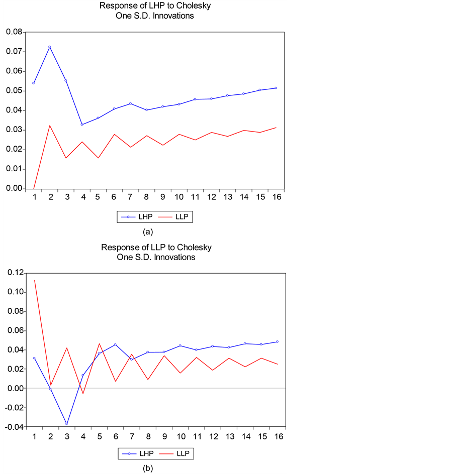
Figure 2. The impulse response function of housing price and land price.
VAR model had on the other variables, while the variance decomposition is used to evaluate the importance of different structural shocks by analyze the contribution of each structural shock to the change of variables. Variance decomposition results of housing price and land price are shown in Table 4 and Table 5.
From the results of variance decomposition of housing price from Table 4 we can see that the change of housing price became stable after the tenth period, more than 78% of them are caused by their own changes, and the shorter the lag phase is, the stronger the explanatory ability of housing price will be; The impact of land price changes had on the housing price change is about 22%. It can be seen that the changes of housing price itself have a major impact on housing price, the change of land price is a minor factor in the change of housing price.
From the results of variance decomposition of land price from Table 5 we can
Table 4. Variance decomposition results of housing price.
Table 5. Variance decomposition results of land price.
see that the impact of housing price changes had on land price had been steadily rising and reached 49.5% in the sixteenth period, while the impact of land price changes had on itself had been declining, till sixteenth period the impact from land price itself was about 50.5%. Relatively, the main influence factor of land price change in the short time is the change of land price itself; in the long run,
changes of housing price and land price had the similar impact on land price changes.
4. Empirical Results Analysis, Conclusions and Policy Recommendations
4.1. Empirical Result Analysis
The result of co-integration test and error correction model shows that there is a stable equilibrium relationship between housing price and land price in Shenzhen. In the long term, the relationship between housing price and land price in Shenzhen is a one-way causal relationship, housing price is the Granger reason of land price, land price is only the result of housing price; in the short term, there exists a Granger cause and effect relationship between housing price and land price.
From the impulse response function we can find the dynamic process of the interaction between housing price and land price: 1 unit impact that housing price had on housing price itself are all positive, while the impact had on land price showed great fluctuations in the short time and exist both positive effects and negative effects. 1 unit impact that land price had on housing price showed large fluctuation in the short time and it gradually became stable after the fifth period, while the impact that land price had on itself are positive expect the third period.
We can have a further understanding of the impact intensity between housing price and land price by variance decomposition. In terms of mutual influence, in the short term, both the contribution of housing price changes to land price changes and the contribution of land price changes to housing price changes are all about 15%; in the long run, the contribution degree that housing price had on land price is almost 50% while the contribution degree that land price had on housing price has been hovering around 20%. In terms of its own influence, the contribution degree that housing price had on itself is about 85% in the short term and 78% in the long term; the contribution degree that land price had on itself is about 85% in the short term and 50% in the long term.
Above all we can see the result of impulse response and variance decomposition support the previous research conclusion. There is a stable equilibrium relationship between housing price and land price in Shenzhen. In the long run, housing price is the Granger reason of land price; in the short term there exist a Granger cause and effect relationship between housing price and land price. At the same time, housing price and land price in Shenzhen are greatly affected by their own changes.
At this stage, the proportion of land price in the real estate of Shenzhen is not large, the main factor that affect the housing price is the market supply and demand. With the continuous development of economy, the continuous increase of income and the continuous inflow of population of Shenzhen in recent years, the real estate market has brought a lot of regid demand to the real estate market, thus pull the short term and long-term tendency of the housing price. The rise in housing price has further raised the developer’s expectations of future income of the land, thus causing the real estate business to increase investment and expand supply, and lead to an increase in demand of land market, eventually led to the rise in land price. Thus it can be seen that the supply of land, land price, housing price and housing supply increased as the demand for housing increased. But in the short term, there are many factors that affect the land supply, such as the adjustment of land supply and the change of supply mode, these will cause the short-term fluctuation of land price, and fluctuations of land price will cause the fluctuations of consumer’s expectations for housing price, thus transmit the impact to the housing price and then result in the short-term fluctuations of housing price.
Another important feature of housing price and land price in Shenzhen is that they are greatly affected by their own change, which is mainly determined by the financial attributes of the real estate. The scarcity of land resources and the long-term rising trend of real estate price have led to the rising expectation of housing price and investment demand for the residents and investors. Real estate is no longer a simple commodity, but turned into a financial asset, which has exceeded the function of living, and become a hard currency, which has the ability to maintain the future purchasing power. In this case, the investment properties of real estate has become particularly prominent. Take the rising real estate as an investment product, even if it can’t make a substantial profit, it can at least achieve wealth preservation. So once the rising expectation of asset has formed, this expectation will be further strengthened in a loose financial environment, and cause the price to rise again, thus form a rising cycle.
4.2. Conclusions and Policy Recommendations
This paper uses the quarterly data of housing price and land price of Shenzhen from 2003 to 2015 to establish error correction model and VAR model, and then makes a study on the relationship between housing price and land price by using impulse response function and variance decomposition. The conclusions are as follows:
1) There is a stable equilibrium relationship between housing price and land price in Shenzhen. In the long run, housing price is the Granger reason of land price; in the short term, there exists a Granger cause and effect relationship between housing price and land price.
2) Housing price and land price in Shenzhen are greatly affected by their own changes. Real estate is no longer a simple commodity, its financial attributes are becoming more and more prominent, and the investment demand has become increasingly large.
According to the research conclusion, in order to make the real estate market develop steadily and healthily, we give the following policy recommendations:
1) Develop a diversified and multi-level real estate market structure system. Not only provide fully residential property, but also provide rental housing; both provide high-grade residential, general residential, and provide affordable housing, low-cost housing. Actively expand the supply channels of the real estate market, and meet the diverse needs of different groups, thus to avoid consumers get together to promote the housing price.
2) Establish land reserve system and make rational land supply planning, strictly enforce the “bid invitation, auction and listing” policy of profit-making land, severely crack down the behavior that disturb the land market. Regulate and control the supply of land to ensure the effective supply of future housing sales market.
3) Improve the dynamic monitoring information system of housing price and land price, public trade information of the real estate market and make an analysis and forecast based on the market data in time, so that to stabilize the psychological expectations of consumers and introduce the consumers to make informed decision.
4) Regulate the investment loan interest rate of real estate and the proportion of self-raised capital, influence the real estate investment market, control the total development and the projects’ types of real estate, and thus regulate the real estate in the supply side.
5) Regulate the interest rate and take measures to limit property-purchasing and loans in the real estate consumption market, restrain speculation behavior in the estate business, balance the contradiction between supply and demand, so that to control the operation and development of the real estate market.
Cite this paper
Wen, Z.Q. (2017) Study on the Dynamic Relationship between Housing Price and Land Price in Shenzhen Based on VAR Model. Journal of Service Science and Management, 10, 28- 42. https://doi.org/10.4236/jssm.2017.101003
References
- 1. Li, C.H. and Wang, Y.Q. (2016) Real Estate Blue Book: Chinese Real Estate Development Report. Social Sciences Academic Press, Beijing.
- 2. Zhang, T.L. (2010) Granger Causality Test of Housing Price and Land Price—An Empirical Research Based on Real Estate Market in China (1998-2009). Chinese Journal of Management Science, 18, 305-311.
- 3. Kuang, W.D. (2005) Research on the Relationship between House Price and Land Price: Model and Chinese Data Test. Finance & Trade Economics, 11, 54-64.
- 4. Song, B. and Gao, B. (2007) Causal Relationship Test between House Price and Land Price: 1998-2006. Modern Economic Science, 1, 72-77.
- 5. Long, H.M. and Guo, W. (2009) Analysis on the Relationship between Housing Price and Land Price in China by VAR Model. Mathematics in Economics, 2, 52-58.
- 6. Sun, B. (2010) The Mechanism and Consequences of High Land Price and High Housing Price. Study and Exploration, 2, 146-148.
- 7. Gao, B. and Mao, F.F. (2003) Empirical Test on the Relationship between House Price and Land Price: 1999~2002. Industrial Economics Research, 3, 19-22.
- 8. Huang, J.B., Jiang, F.T. and Chen, W.G. (2007) The Re-Examination of the Relationship between House Price and Land Price in China. Forecast, 2, 1-7.
- 9. Xu, Y. (2002) The Reason Why the Housing Price in Beijing Are So High and Control of Housing Price. Urban Problems, 1, 42-44.
- 10. Dowall, D.E. (1982) Land-Use Controls and Housing Costs: An Examination of San Francisco. Areuea Journal, 10, 67-93.
https://doi.org/10.1111/1540-6229.00258 - 11. Liu, L. and Liu, H.Y. (2003) Economic Analysis of the Relationship between Land Price and House Price. The Journal of Quantitative & Technical Economics, 7, 27-30.
- 12. Yan, J.H. (2006) Housing Price and Land Price in China: Theoretical, Empirical and Policy Analysis. The Journal of Quantitative & Technical Economics, 1, 17-26.
- 13. Huang, J. and Tu, M.Z. (2009) Empirical Analysis on the Relationship between Urban Housing Price and Land Price in China Based on Non-Stationary Panel. Statistical Research, 7, 13-19.
- 14. Granger, C.W.J. (1988) Some Recent Development in Concept of Causality. Journal of Econometrics, 39, 199-211.
https://doi.org/10.1016/0304-4076(88)90045-0 - 15. Gao, T.M. (2007) Econometric Methods and Modeling. Tsinghua University Press, Beijing.
- 16. Liu, L. (2004) Interaction Mechanism and Policy Analysis of Real Estate Market. Economic Press, Beijing.
- 17. Zheng, L. and Chen, L.W. (2016) Regional Comparison of the Impact of Monetary Policy on House Prices. Business Economic Research, 1, 159-161.