Natural Science
Vol.12 No.05(2020), Article ID:100146,25 pages
10.4236/ns.2020.125022
Potential Power of the Pyramidal Structure II
Osamu Takagi1, Masamichi Sakamoto2, Hideo Yoichi1, Kimiko Kawano1, Mikio Yamamoto1
1International Research Institute (IRI), Chiba, Japan; 2Aquavision Academy, Chiba, Japan
Correspondence to: Osamu Takagi, 
Copyright © 2020 by author(s) and Scientific Research Publishing Inc.
This work is licensed under the Creative Commons Attribution International License (CC BY 4.0).
http://creativecommons.org/licenses/by/4.0/


Received: April 7, 2020 ; Accepted: May 10, 2020 ; Published: May 13, 2020
ABSTRACT
Research on “pyramid power” began in the late 1930s. To date, many documents on “pyramid power” have been published. We have been conducting scientific research on the unexplained “power” of a pyramidal structure (PS) since October 2007. The research focuses on the detection of a non-contact effect of the unexplained “power” of the PS on biosensors (i.e., edible cucumber sections of Cucumis sativus “white spine type”) placed at the top of the PS. In this paper, in particular, we compared the non-contact effect of upper and lower biosensors placed in two layers on the PS apex, and we analyzed the difference of the non-contact effect due to the difference in the layers. The magnitude of the non-contact effect was represented by the calibrated psi index Ψ(E-CAL) calculated from gas concentrations emitted from the biosensors. A method to determine the presence or absence of the non-contact effect by analyzing the gas concentrations was developed by the International Research Institute (IRI). Ψ(E-CAL), which represents the magnitude of the non-contact effect, was the average value of the respective non-contact effect of the upper and lower biosensors stacked in two layers on the PS apex. We conducted the analysis on the assumption that the non-contact effect on the upper and lower biosensors might be different. Therefore, we considered that upper and lower biosensor calibration was required for Ψ(E-CAL), and we introduced a new calibrated psi index Ψ(E-CAL)Layer. Scientifically rigorous experiments to date have detected Ψ(E-CAL) with statistical significance and have demonstrated potential power of the PS (p = 6.0 × 10⁻³; Welch’s t-test, two-tails, the following p values are also the Welch’s t-test values). Based on data demonstrating the potential power of the PS, we analyzed the non-contact effects on the upper and lower biosensors of the PS apex. We obtained a surprising result that the non-contact effect on the upper biosensors (farther from the PS) was larger than that on the lower biosensors (closer to the PS) (p = 4.0 × 10⁻⁷). This suggested that the characteristic of the potential power of the PS, which is considered to exist near the PS apex, is distinctive. We also found that the non-contact effect due to the potential power of the PS varies with the season, and is large in summer and small in winter. In our discussion, we proposed a model that could theoretically explain the experimental results that the non-contact effect on the upper biosensors at the PS apex is larger than the lower biosensors. In proposing this model, we assumed that there were two different types of potential power at the PS apex and that the biosensors had two different gas-generating reactions. In a simulation using the model, the experimental results were well approximated in which the non-contact effect on the biosensors differs depending on the difference between the upper and lower layers. The results of this paper are the world’s first to prove aspects of the “pyramid power” through scientifically rigorous experiments and analysis. These results will become a new field of science in the future, and their broad applications are expected.
Keywords:
Pyramid, Potential Power, Meditation, Unconsciousness, Non-Contact Effect, Delay, Biosensor, Cucumis sativus, Gas

1. INTRODUCTION
In the late 1930s, the Frenchman Antoine Bovis found a naturally mummified small animal in the Great Pyramid of Giza. This was the beginning of research on a so-called “pyramid power”. To date, many documents on the “pyramid power” have been published [1-18]. Among them, some made a scale model of the large pyramid of Giza and conducted experiments [1-4,8,12,18], one book tried to elucidate unexplained functions of the pyramid using mathematical formulas [17], and another acquired patent information [15]. However, scientific research papers published in academic journals are rare [19,20]. On the other hand, it is true that there are documents that deny the existence of the “pyramid power” as pseudo-science [21-24]. The grounds for denying the “pyramid power” are that experiments did not provide sufficiently statistical significance, and that there was no scientific theory to understand the phenomenon.
We have been studying unexplained “power” of a pyramidal structure (PS) using a biosensor (edible cucumber sections: Cucumis sativus “white spine type”) since October 2007. Scientifically rigorous experiments and analyzes demonstrated the existence of an unexplained “power” of the PS (an unexplained function of the PS) with statistically very high significance. The results of our research on the PS have been published as seven original papers [25-31], two research summaries [32,33], and one chapter in a book [34].
In experiments using the PS, we performed two types of experiments with different conditions as follows.
Experiment 1: An experiment conducted in a state where the PS and a human (a test subject) were related.
Experiment 2: An experiment conducted in a state where the PS and a human (a test subject) were not related.
Experiment 1 is the experiment that was conducted from several hours before meditating to 20 days after meditation when the test subject meditated (Hemi-Sync® [35]) within the PS. Experiment 1 suggested the existence of two unexplained energies of human origin (force types I and II) [31,33]. From Experiment 1, the following two results were obtained.
1) When the PS and a human unconsciousness (force type I) were related.
A change in the non-contact effect, which seems to correspond to an unconscious change, was detected during the transition from a sleep state to an awake state of a human (the test subject) 6 km or more away (1% significance) [30,33].
2) When the PS and the effect of a human (the test subject) meditating in the PS (force type II) were related.
The non-contact effect with delay was detected over a dozen days after meditation (p = 3.5 × 10⁻⁶; Welch’s t-test, two-tails, the following p values are also the Welch’s t-test values) [26,27,32,33]. The characteristics of the non-contact effect with delay could be very well approximated by theoretical curves calculated from a model of transient response phenomena in control theory [26,32,33].
As a result of Experiment 2, the non-contact effect on the biosensors placed at the PS apex was detected with statistical significance (p = 6.0 × 10⁻³), demonstrating the existence of the potential power of the PS [31]. It was also found that the non-contact effect due to the potential power of the PS varies with the season, and is large in summer and small in winter.
Until now, the non-contact effect on the biosensors has been expressed as the calibrated psi index Ψ(E-CAL) [31,34]. Ψ(E-CAL) is the average value of the non-contact effect values Ψ1(E-CAL) and Ψ2(E-CAL) of the upper and lower biosensors placed on the PS apex in two layers. In this paper, based on the experimental data obtained in Experiment 2, the non-contact effect of each of the upper and lower biosensors placed at the PS apex was compared. Therefore, we considered that upper and lower sensor calibration is required for Ψ(E-CAL), and we introduced a new calibrated psi index Ψ(E-CAL)Layer. The reason that the introduction of Ψ(E-CAL)Layer became possible was that sufficient experimental data were obtained (n = 468), and analysis that separated the upper and lower layers became possible. A surprising result was obtained that the non-contact effect on the upper biosensors (farther from the PS) was larger than that of the lower biosensors (closer to the PS) (p = 4.0 × 10⁻⁷). In other words, it became clear that the potential power of the PS has different effects on the upper and lower biosensors. In order to understand this phenomenon quantitatively, we improved the model proposed in our previous paper [31] and proposed a new model considering the distribution characteristics of potential power of the PS. In a simulation using this new model, we were able to approximate the experimental results in which the non-contact effect differs between the upper and lower layers. The discovery of the potential power of the PS obtained through scientifically rigorous experiments and analysis is the world’s first research to demonstrate the “pyramid power”. This result will become a new field of science in the future, and broad applications are expected.
2. EXPERIMENT
2.1. Pyramidal Structure (PS)
Figure 1(a) showed the PS used in the present experiment. The PS was a square pyramid with a height of 107 cm, a ridgeline length of 170 cm and a base length of 188 cm. The angle (tilt angle) between the bottom and the side of the PS was 49.1˚. The base of the PS was raised by four tripods to a height of 73 cm from the floor. The frame of the PS was made of four aluminum pipes (2 cm diameter, 0.36 cm thick pipe wall). Each side had a Sierpinski triangle pattern and it consisted of aluminum plates (0.3 mm thick). At the top of the PS, a Faraday cage for electrostatic shielding of the biosensors was placed. A calibration control point was set up 8 m away from the PS [25,34]. The PS is a simple and static structure which does not have any mechanically movable parts nor does it have a supply of known energy.
2.2. Detection of Unexplained “Power” (Non-Contact Effect) of the PS
To demonstrate the “pyramid power” of the PS, we examined the presence or absence of the non- contact effect on the biosensors (cucumber fruit sections). To detect the non-contact effect, the gas concentration generated by the gas production reaction of the cucumber sections was measured. Samples were prepared according to a simultaneous calibration technique (SCAT) [36] to prepare homogeneous biosensors (Figure 1(b)). The detection method the non-contact effect by analyzing the gas concentrations released from the biosensors was researched and developed by the International Research Institute (IRI),
and we used it previously to successfully detect a healer’s non-contact effect and a wave like bio-field around the healer [37-39].

Figure 1. Pyramidal structure used in the experiment, biosensors and its installation status. (a) shows the pyramidal structure (PS) used in the experiment. (b) Left, biosensors prepared according to SCAT; right, placement of samples on the PS apex and calibration control point for the PS. (c) Left, placement of samples at the PS apex; right, placement of samples at the PS apex and calibration control point (pattern diagram).
GE1 and GE2, the experimental samples of Pair 1 and Pair 2 in Figure 1(b), were placed in covered Petri dishes at the PS apex in two layers. And GC1 and GC2, the control samples of Pair 1 and Pair 2, and GE3, GE4, GC3 and GC4, the control samples of Pair 3 and Pair 4 were similarly placed at the calibration control point 8 m away from the PS, also in two layers. For GE and GC, the larger subscript number was the upper layer (Figure 1(c)). The biosensors were kept in place for 30 minutes. GE and GC were the same cut section, but the direction of the cutting was different. GE was cut in the same direction as the cucumber growth axis, while GC was cut in the opposite direction. Previous experiments demonstrated that the gas concentration varies depending on the direction of the cut section, and GE < GC [29]. The center point of the bottom of the Petri dish of GE1 placed at the PS apex coincided with the extension of the center of the four aluminum pipes near the PS apex (Figure 1(c)). After setting the covered Petri dish there for 30 minutes, the Petri dish was removed from the PS and its lid was taken off. Each Petri dish was then placed in a closed container with a volume of 2.2 liters and the containers were placed in a temperature-controlled room to be stored side by side on shelves for each pair. Storage time was 24 h-48 h. After storage, the gas concentrations released from the cucumber sections were measured. Gas detection tubes (Ethyl acetate detector tube 141 L: Gastech, Japan) and a gas sampling pump (GV-100: Gastech, Japan) were used to measure the gas concentrations.
2.3. Non-Contact Effect Magnitude Psi Index Ψ
To examine the non-contact effect on the biosensors, we introduced a psi index Ψ that quantifies the magnitude of the non-contact effect [31,34]. Ψ was calculated by Equation (1) using the measured gas concentrations. We considered that the unexplained “power” of the PS has a very small effect on changes in gas concentrations. Then, the non-contact effect may be buried in noise, making its detection difficult. The reason was that the gas generation reaction of the biosensors was considered to react sensitively due to factors such as differences between individual cucumbers and environmental conditions. Therefore, in order to minimize the noise displacement, a paired sample method (Figure 1(b)) was used in which GE and GC were compared as a pair. Ψ is 100 times the natural logarithm of the ratio calculated for the gas concentrations of each pair. The relationship between the J value we used previously and Ψ was Ψ = 100 J [40].
(1)
In Equation (1), GE1-GE4 and GC1-GC4 were gas concentrations (ppm) measured from the biosensors shown in Figure 1(b). Ψ1-Ψ4 were the psi index values before calibration. GE3, GC3, GE4, and GC4 were biosensors placed at the calibration control point, and GE and GC differed only in the direction of the cut section. Therefore, it was considered that the influence of the difference in the direction of the cut section of cucumber was detected from Ψ3 and Ψ4. From Ψ1 and Ψ2, it was considered that two effects were detected, the effect of the difference in the cutting direction and the effect of the difference in the placement (the PS apex and the calibration control point). The results of subtracting the average values of Ψ3 and Ψ4 from Ψ1 and Ψ2 are Ψ1(E-CAL) and Ψ2(E-CAL). Ψ1(E-CAL) and Ψ2(E-CAL) calibrated against environmental factors such as temperature, humidity, atmospheric pressure, geomagnetism, etc., and also calibrated against the cutting direction. Therefore, the calibrated psi indices, Ψ1(E-CAL) and Ψ2(E-CAL), were considered to be the results (non-contact effect by the PS) reflecting only the effect of the unexplained “power” of the PS.
(2)
Finally, the calibrated psi index Ψ(E-CAL), the non-contact effect on the biosensors, was obtained from the average of the lower and upper calibrated psi indices Ψ1(E-CAL) and Ψ2(E-CAL).
(3)
The purpose of this paper was to analyze the difference of the non-contact effect on the upper and lower biosensors placed in two layers. Therefore, Ψ(E-CAL)Layer was introduced, which allows calibration of the two stacked upper and lower layers.
(4)
Here, Ψ(E-CAL)LayerAve, which is the average value of Ψ1(E-CAL)Layer1 and Ψ2(E-CAL)Layer2, coincided with Ψ(E-CAL).
(5)
3. EXPERIMENTAL AND ANALYTICAL RESULTS
In this paper, in order to verify the potential power of the PS, the data obtained in Experiment 2 described in “1. Introduction” were analyzed (n = 468). Experiment 2 was not only an “experiment performed without the test subject in the PS”, but also an experiment that met two conditions (Conditions 1 and 2). The reason why these conditions were added is described below. If Conditions 1 and 2 were not satisfied, we had found that the effect of the PS on the biosensors was not the effect of the potential power of the PS but the effect of “the state in which the PS and the test subject were related” [26,27,30,32,33].
Figure 2 shows the average gas concentration released from the biosensors (n = 468). In the figure, we observed no significant difference between the average gas concentrations of all the biosensors GE1-GE4 and GC1-GC4 (p = 0.088). However, the following possibilities 1)-4) were considered. 1) At the PS apex, the gas concentration of the biosensors placed in the upper layer (GE2) was higher than that in the lower layer (GE1). 2) Conversely, at the calibration control point, the gas concentrations of the biosensors placed in the upper layer (GE4, GC2, GC4) were lower than those in the lower layer (GE3, GC1, GC3). 3) When the experimental sample GE1-GE4 and the control sample GC1-GC4 were compared, the difference in gas concentration due to the layer was larger in GE1-GE4 than in GC1-GC4. 4) In the experimental samples, the

Figure 2. Average gas concentration emitted from the biosensors. The red circles indicate the average gas concentrations of the biosensors GE1 and GE2 placed at the PS apex. The blue circles indicate the average gas concentrations of the biosensors GE3, GE4 and GC1-GC4 placed at the calibration control point. The results of the two stacked biosensors are connected by dotted lines. All error bars show the 99% confidence interval.
difference in gas concentration due to the difference in layer was reversed between GE1 and GE2 at the PS apex and GE3 and GE4 at the calibration control point. 5) In the control samples, GC1, GC2, GC3 and GC4 at the calibration control point showed almost equal changes in gas concentration due to the difference in the layer. From 1)-5), it was considered that the biosensors GE1 and GE2 at the PS apex showed an abnormal reaction as compared with the biosensors at the calibration control point.
Figure 3 shows a scatter plot (n = 468) to determine whether there was a correlation between the gas concentrations emitted from the biosensors stacked in two layers, upper and lower. It was concluded that the correlation coefficient of gas concentration between the two layered biosensors was about 0.7 at both the PS apex and the calibration control point, indicating a positive correlation.
Figure 4(a) shows the sum of the gas concentrations of the upper and lower biosensors in two layers.
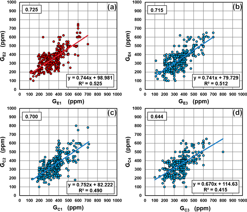
Figure 3. The scatter plot of gas concentration of the biosensors placed in two layers, upper and lower. The vertical axis shows the results of the upper layer biosensors and the horizontal axis shows the results of the lower layer biosensors. (a) shows the results of the biosensors placed at the PS apex. (b)-(d) show the results of the biosensors placed at the calibration control point. The numerical value at the upper left of each graph is the correlation coefficient. The lower-right part of each graph shows the first-order approximation fitting line and the coefficient of determination R2.

Figure 4. Sum and ratio of the gas concentrations. (a) The sum and (b) the ratio of the gas concentrations of the upper and lower biosensors in a two-layered biosensor. All error bars show the 99% confidence interval.
From an analysis of variance (ANOVA), p = 0.45 and no significant difference was observed. However, different gas concentrations (GE < GC) were obtained depending on the direction of the axis of the cut section of the cucumbers [29]. The experimental samples (GE1 + GE2) and (GE3 + GE4) were almost the same, but the control samples tended to be in the order (GC1 + GC2) < (GC3 + GC4). The following was considered as the reason for this order despite being placed at the calibration control point and having the same axial direction for cutting. In other words, we considered that the effect of the PS apex did not appear directly on the biosensors GE1 and GE2 placed at the PS apex, rather it appeared on the biosensor pair GC1 and GC2. A similar phenomenon has been seen in other experimental reports [39,41]. Figure 4(b) shows the gas concentration ratio calculated by dividing the upper gas concentration by the lower one, taking the logarithm and multiplying by 100. This expression was similar to the psi index of Equation (1). For ANOVA, p = 5.2 × 10⁻⁶, and a significant difference was recognized. Tukey’s test showed that 100ln(GE2/GE1) was abnormally large compared to the others. Figure 4 revealed the following findings. No significant difference was found in the sum of the gas concentrations of the biosensors placed on the upper and lower layers, but the ratio of the gas concentrations indicated that 100ln(GE2/GE1) was abnormally large. Therefore, it was considered that one or both GE1 and GE2 placed at the PS apex exhibited an abnormal change different from that when placed at the calibration control point.
Figure 5 shows the scatter diagram (n = 468) to determine whether or not there is a correlation between the gas concentrations of the biosensors of the pair shown in Figure 1(b). Figure 5(a) and Figure 5(b) include the results of GE1 or GE2 placed at the PS apex. Figure 5(c) and Figure 5(d) include the results of the biosensors placed at the calibration control point. All the correlation coefficients showed a positive correlation of about 0.8. Therefore, it was found that the correlation coefficient between the paired biosensors was larger than the correlation coefficient between the two layered biosensors in Figure 3.
Figure 6(a) shows the average (n = 468) of the sum of the gas concentrations emitted from the

Figure 5. The scatter plot of gas concentration of the biosensors between pairs. The vertical axis indicates results of the experimental samples (GE), and the horizontal axis indicates results of the control samples (GC). (a) and (b) show the results including GE1 and GE2 placed at the PS apex. (c) and (d) show the results of the biosensors on the calibration control point. The numerical value at the upper left of each graph is the correlation coefficient. The lower-right part of each graph shows the first-order approximation fitting line and the coefficient of determination R2.
biosensors of the pair. For ANOVA, p = 0.57, and no significant difference was observed. Although there was no significant difference, when (GE3 + GC3) and (GE4 + GC4) placed at the calibration control point were compared, there was a tendency that (GE3 + GC3) > (GE4 + GC4). The difference between (GE3 + GC3) and (GE4 + GC4) was only the difference between the respective upper and lower layers. Therefore, at the calibration reference point, it was suggested that the gas concentration of the lower biosensors was higher than that of the upper biosensors. Atmospheric pressure was considered as one of the causes. On the other hand, when (GE1 + GC1) and (GE2 + GC2) including the biosensors GE1 and GE2 placed at the PS apex were compared, the opposite tendency was shown. Similar to the results of Figure 2 and Figure 4(b), the following was found from the results of Figure 6(a). GE1 and GE2 placed at the PS apex were abnormal compared to GE3, GE4 and GC1-GC4 at the calibration control point. However, it was not possible to determine

Figure 6. Sum of gas concentration of paired biosensors and psi index Ψ1-Ψ4. (a) shows the average of the sum of the gas concentrations of the biosensors in the pair shown in Figure 1(b). (b) shows the psi index Ψ1-Ψ4 calculated by Equation (1). All error bars show the 99% confidence interval.
whether the abnormality was with GE1 or GE2, or both. Therefore, we tried to identify them separately by calculating the psi index Ψ1-Ψ4 (Figure 6(b); the vertical axis is the magnitude of the psi index, and the horizontal axis is the psi index Ψ1-Ψ4 before the calibration calculation by Equation (1)). For ANOVA, a significant difference was obtained for Ψ1-Ψ4 (p = 9.3 × 10⁻⁶). Among Ψ1-Ψ4 values, only Ψ2 was positive and the others were negative. There was no significant difference between Ψ1, Ψ3 and Ψ4. Therefore, Ψ2 was considered to indicate an abnormal value. Since GE2 was included in the formula of Ψ2, we concluded that GE2 placed at the PS apex showed an abnormal value different from other biosensors. However, there was no significant difference between Ψ1, Ψ3 and Ψ4, but it seemed that there was a difference between Ψ3 and Ψ4. The cause was thought to be the result of the difference due to the layer between the pairs, as pointed out in the explanation of Figure 6(a).
Figure 7(a) and Figure 7(b) show the moving average (window size is 180 days) of psi index Ψ1-Ψ4. The horizontal axis indicates the dates which are values from 1 to 366 obtained by starting at 1 and counting from January 1 of each year in which the experiment was conducted. The dates analyzed in this paper were obtained from experiments between July 2010 and September 2017. Using the same experimental data, we have already published one paper demonstrating the potential power of the PS [31]. In addition, papers on the unexplained functions of the PS [26,27,30] and papers on the characteristics of the biosensors [28,29] were presented from the results of experiments conducted during the same period. From the results of the moving averages of Ψ1 and Ψ2 (Figure 7(a)), we found that Ψ1 < Ψ2 throughout the year, with the psi index increasing in summer and decreasing in winter. Summer was the period when the daytime was more than 12 hours and therefore from the day of the spring equinox to the day of the autumn equinox. When not a leap year, the former was March 20, and the value on the horizontal axis, 81. Similarly,

Figure 7. Moving average of psi index Ψ1-Ψ4. (a) and (b) are moving averages of the psi index Ψ1-Ψ4 (window size is 180 days). The horizontal axis is the date (1-366). The solid line is the psi index calculated from the lower layer pair, and the dotted line is the psi index calculated from the upper layer pair.
the latter was September 23, and the value on the horizontal axis, 267. Winter was the period when the daytime was less than 12 hours. The numbers of summer data were n = 252 and for winter data, n = 216. In Figure 7(b), the moving averages of Ψ3 and Ψ4 were both negative values, which could be understood from the result of GE < GC [29]. The moving averages of Ψ3 and Ψ4 were considered to be almost constant throughout the year. In Figure 7(a), Ψ1 < Ψ2 for the lower layer Ψ1 and the upper layer Ψ2, whereas in Figure 7(b), Ψ3 > Ψ4 for the lower layer Ψ3 and the upper layer Ψ4. In other words, we found that the magnitude of the psi index showed the opposite tendency between Figure 7(a) and Figure 7(b). Similar to the previous results, the results in Figure 7 also showed that the PS apex is a space that gives a unique effect (non-contact effect) to the biosensors compared to the calibration control point. Based on the results of the calibration control point, we found that Ψ1 tended to decrease in winter and Ψ2 tended to increase in summer.
Figure 8(a) shows the scatter plot for Ψ1 and Ψ2, and Figure 8(b) shows the scatter plot for Ψ3 and Ψ4. It was found that both Figure 8(a) and Figure 8(b) had a positive correlation. As seen in Figure 5, the correlation between the gas concentrations of the pairs was about 0.8 in all cases, and the distribution was similar. In contrast, the following was found from the scatter plot of Ψ calculated from the ratio of the gas concentrations of the pair. The distributions of Ψ1 and Ψ2 that included the gas concentration at the PS apex and the distributions of Ψ3 and Ψ4 that included the gas concentration at the calibration control point were significantly different. The results in Figure 8 also revealed that the PS apex was a space that showed an abnormal response to the biosensors compared to the calibration control point.
Figure 9 shows the difference in the non-contact effect due to the difference in layers for the biosensors

Figure 8. The scatter plot of psi index. (a) is a scatter plot of Ψ1 and Ψ2. (b) is a scatter plot of Ψ3 and Ψ4. The numerical value at the upper left of each graph is the correlation coefficient. The lower part of the graph shows the linear approximation fitting line and the coefficient of determination R2.
placed at the PS apex (n = 468). Above, Figure 6(b) and Figure 7(a) suggested that the magnitude of the non-contact effect on the biosensors placed at the PS apex differs between the upper and lower layers. Figure 9 shows in two ways the non-contact effect on the upper and lower biosensors located at the PS apex; that is, Ψ(E-CAL) and Ψ(E-CAL)Layer which can calibrate the difference between layers. The black circles show the average value of Ψ1(E-CAL) and Ψ2(E-CAL) in Equation (2) (p = 2.5 × 10⁻⁵). The red squares show the average value of psi index which was calibrated for the difference in the layers in Equation (4)., Ψ1(E-CAL)Layer1 = Ψ1-Ψ3 and Ψ2(E-CAL)Layer2 = Ψ2-Ψ4 (p = 4.0 × 10⁻⁷). It was found that the Ψ(E-CAL)Layer, which calibrated the layer difference, had a smaller p-value than Ψ(E-CAL). From these results, we concluded that it was necessary to use the Ψ(E-CAL)Layer that calibrated the difference between layers when analyzing the difference between the upper and lower layers of the non-contact effect on the biosensors placed at the PS apex.
Figure 10(a) shows the moving average (window size is 180 days) of Ψ1(E-CAL)Layer1, Ψ2(E-CAL)Layer2 and their average Ψ(E-CAL)LayerAve. According to Figure 9, for the average value, Ψ1(E-CAL)Layer1 < Ψ2(E-CAL)Layer2. And from Figure 10(a), the tendency of Ψ1(E-CAL)Layer1 < Ψ2(E-CAL)Layer2 was seen throughout the year. At the PS apex, the non-contact effect on the upper biosensors was larger than on the lower biosensors. The Ψ1(E-CAL)Layer1 and Ψ2(E-CAL)Layer2 tended to increase in summer and decrease in winter. Figure 10(b) shows the scatter diagram of Ψ1(E-CAL)Layer1 versus Ψ2(E-CAL)Layer2. The correlation coefficient was 0.87, indicating a strong correlation.
Figure 11 shows the summer and winter data for Ψ1-Ψ4 and Ψ1(E-CAL)Layer1, Ψ2(E-CAL)Layer2. Earlier, Figure 6(b) showed the annual average of Ψ1-Ψ4, while Figure 11(a) shows the average of summer and winter values of Ψ1-Ψ4. The number of data was n = 252 in summer (orange squares) and n = 216 in winter (black squares). Compared to the difference between summer and winter of Ψ3 and Ψ4 calculated only with the biosensors placed at the calibration control point, it was found that the difference between summer and winter of Ψ1 and Ψ2 including GE1 and GE2 placed at the PS apex was larger. This result was expected

Figure 9. The non-contact effect on the biosensors placed at the PS apex in two layers. The black circles are the average value of the calibrated psi indices Ψ1(E-CAL) and Ψ2(E-CAL) in Equation (2). The red squares are the average values of the psi index Ψ1(E-CAL)Layer1 = Ψ1-Ψ3 and Ψ2(E-CAL)Layer2 = Ψ2-Ψ4, which was calibrated for the difference in the layers in Equation (4). All error bars show the 99% confidence interval.
from Figure 7(a) and Figure 7(b). Although the reason is not clear, there was a tendency that Ψ3 > Ψ4 at the calibration control point. Figure 11(b) shows the summer and winter data of Ψ1(E-CAL)Layer1 and Ψ2(E-CAL)Layer2 with respect to the results of Figure 9. It turned out that summer and winter behaviors were the consequence of almost parallel movement.
4. Discussion
4.1. Moving Average of the Ψ(E-CAL) and Proposal of “Model 1”
In our previous paper [31], we conducted the demonstration of the potential power of the PS under the condition that “the PS and a human (the test subject) were not related”. As a result, the average value of the Ψ(E-CAL), which indicates the magnitude of the non-contact effect, became a positive value in summer, demonstrating the potential power of the PS (1% significance). It was also found that the moving average of the Ψ(E-CAL) changed seasonally. We introduced one theoretical model that can explain the seasonal change of the moving average of the Ψ(E-CAL) (“Model 1”) [31]. The introduction process of “Model 1” is shown in 1) to 3) below.
1) Data analysis revealed that the moving average of Ψ(E-CAL) was large in summer and small in winter.
2) “Model 1” was introduced to explain the seasonal change of the moving average of the Ψ(E-CAL) (Figure 12). The characteristics and assumptions of “Model 1” were as follows (i)-(iv).
(i) There are two types of potential powers (potential power 1 (P1) and potential power 2 (P2)) near the PS apex.
(ii) The biosensors GE1 and GE2 at the PS apex are affected by the potential powers P1 and P2.

Figure 10. The moving average of Ψ1(E-CAL)Layer1,Ψ2(E-CAL)Layer2 and their average, and the scatter plot of Ψ1(E-CAL)Layer1 and Ψ2(E-CAL)Layer2. (a) shows the moving average (window size is 180 days) of the psi index Ψ1(E-CAL)Layer1 (red solid line), Ψ2(E-CAL)Layer2 (red dotted line) and their average Ψ(E-CAL)LayerAve (green solid line). (b) is a scatter diagram of Ψ1(E-CAL)Layer1 on the horizontal axis and Ψ2(E-CAL)Layer2 on the vertical axis.
(iii) There are at least two types of biosensor gas generation reactions (α reaction and β reaction).
(iv) In “Model 1”, αE and βE are the average gas concentrations generated from the experimental sample (GE) by α and β reactions. The αC and βC are the average gas concentrations generated from the control sample (GC) by α and β reactions. Further, αE < αC and βE < βC are satisfied. The reason is that the gas concentration varies depending on the axial direction of the cucumber section [29]. To facilitate understanding, αE = βE and αC = βC.
3) The relationships between the potential power of the PS and the gas production reaction were assumed as follows. “In winter, the potential power P1 suppresses gas generation due to the α reaction and the gas concentration decreases by G(P1). As a result, αE of GE1 and GE2 becomes αE(winter). Throughout the year, the potential power P2 facilitates gas generation due to the β reaction and the gas concentration increases by G(P2). As a result, βE of GE1 and GE2 becomes βE(year).”
The introduction process of 1)-3) made it possible to qualitatively understand the moving average of the Ψ(E-CAL). From Equation (5), Ψ(E-CAL) = Ψ(E-CAL)LayerAve. Therefore, the moving average of Ψ(E-CAL) matches the moving average of Ψ(E-CAL)LayerAve (Figure 10(a)). Thus, it was found that the change of the moving average of Ψ(E-CAL)LayerAve can be understood by the PS potential powers P1, P2 and the gas generation reactions α, β. The Ψ(E-CAL)LayerAve is the average of Ψ1(E-CAL)Layer1 and Ψ2(E-CAL)Layer2 that calibrate the difference between the lower and upper layers. Therefore, like Ψ(E-CAL)LayerAve, we thought that the moving average of

Figure 11. Comparison of psi indices between summer and winter. (a) compares the summer and winter seasons for Ψ1-Ψ4 plotted in Figure 6(b). (b) compares the summer and winter seasons for Ψ1(E-CAL)Layer1 and Ψ2(E-CAL)Layer2 plotted in Figure 9. The black squares are winter and the orange squares are for summer.
Ψ1(E-CAL)Layer1 and Ψ2(E-CAL)Layer2 can also be explained by the PS potential powers P1, P2 and gas generation reactions α, β.
4.2. Moving Average of Ψ1(E-CAL)Layer1 and Ψ2(E-CAL)Layer2, and Proposal of “Model 2”
As a result of data analysis, we found that Ψ1(E-CAL)Layer1 < Ψ2(E-CAL)Layer2. The surprising result (p = 4.0 × 10⁻⁷) was obtained that the non-contact effect on the biosensors in the upper layer was larger than that in the lower layer at the PS apex (Figure 9). The reason was considered to be the difference between the upper and lower environments, for example, the difference in brightness and the weight applied to the Petri dish. However, since Ψ(E-CAL)Layer calibrated the difference between the upper and lower environments, the effects due to the environment should have been removed. In order to theoretically understand that the non-contact effect differs depending on the difference between the upper and lower layers, we propose a new “Model 2” that is a modification of “Model 1” (Figure 13 and Figure 14). In “Model 2”, the relationships between potential powers P1, P2 of the PS and gas generation reactions α, β are the same as in “Model 1”. The P1 is distributed near the PS apex in a region including GE1 and GE2. However, P2 is assumed as in the following (i)-(ii).
(i) The P2 spreads out in a cone starting from the PS apex (Figure 13(a) and Figure 13(b)).
(ii) The P2 only affects biosensors inside the cone and does not affect biosensors outside the cone.
According to the assumptions (i)-(ii), P2 affects only a small part of the surface of the four cucumber

Figure 12. Features of “Model 1”. In (a), two types of potential powers P1 and P2 are assumed near the PS apex. Potential powers P1 and P2 affect GE1 and GE2 at the PS apex. In (b), there are at least two types of biosensor gas generation reactions (α reaction and β reaction). The αE and βE are the average gas concentrations generated from the experimental sample (GE) by the α and β reactions. The αC and βC are the average gas concentrations generated from the control sample (GC) by the α and β reactions. In the α reaction, the gas concentration decreases by G(P1) in winter due to P1. In the β reaction, P2 increases the gas concentration by G(P2) throughout the year.
sections in the Petri dish for the lower GE1 (Figure 13(c): lower). On the other hand, it is considered that P2 affects the entire surface of four cucumber sections in the Petri dish for GE2 in the upper layer (Figure 13(c): upper).
Figure 14 shows changes in gas concentrations in summer (Figure 14(a)) and winter (Figure 14(b)) due to the potential powers P1 and P2. In summer, P2 increases the gas concentration of βE of GE2 by G(P2) (βE of GE1 does not change because P2 has almost no effect on GE1). In winter, the effect of P2 is the same as in summer, but the gas concentration of αE of GE1 and GE2 decreases by G(P1) due to P1. The introduction of “Model 2” enables a qualitative understanding of the moving average of Ψ1(E-CAL)Layer1 and Ψ2(E-CAL)Layer2.
4.3. Quantification of αE, αC, βE, βC in “Model 2”
Figure 2 showed the average gas concentration (ppm) of each biosensors GE1-GE4, GC1-GC4, and the average value was (GE1, GE2, GE3, GE4, GC1, GC2, GC3, GC4) = (344.7, 355.5, 356.2, 343.6, 358.5, 351.9, 359.7, 355.7). From these results, it was confirmed that GE1 and GE2 at the PS apex had abnormalities as compared with the biosensors GE3, GE4, and GC1-GC4 placed at the calibration control point. In order to clarify the abnormality of GE1 and GE2, we tried to find the model value of gas concentration based on the gas concentration at the calibration control point. The average gas concentration of the four biosensors GC1-GC4 was 356.5 ppm and the average of GE3 and GE4 was 350 ppm. The average difference between the upper and lower layers was 5 ppm between GC1 and GC4 and 13 ppm between GE3 and GE4. From these results, assuming that the biosensors at the PS apex had the same reaction as the calibration control point, we obtained the model value of the gas concentration as follows: (GE1, GE2, GE3, GE4, GC1, GC2, GC3, GC4) = (356.4, 343.4,

Figure 13. Features of “Model 2”. In (a) and (b), P1 is distributed near the PS apex including GE1 and GE2 as in “Model 1”. It is assumed that P2, unlike “Model 1”, extends conically from the PS apex. In (c), P2 affects only a part of the surface of the four cucumber sections in the Petri dish for GE1 in the lower layer. For the upper GE2, P2 affects the entire surface of the four cucumber sections in the Petri dish.
356.4, 343.4, 359.1, 353.8, 359.1, 353.8). These measured and model values are graphed in Figure 15. When the measured and model values were compared, they almost matched at the calibration control point, but change at the PS apex had the opposite tendency. Figure 16(a) and Figure 16(b) shows the summer and winter gas concentrations of GE1-GE4 and GC1-GC4 based on this model value. As described above, since it was assumed that αE = βE and αC = βC in the gas generation reactions α and β, the values of α and β were half of the model values. As in Figure 14, the gas concentration of βE of GE2 increased by G(P2) in summer. In winter, βE of GE2 increased by G(P2), and αE of GE1 and GE2 decreased by G(P1). Next, the magnitudes of G(P1) and G(P2) were estimated from the measured gas concentration.
4.4. Quantification of G(P1) and G(P2) in “Model 2”
Here, we attempted to quantitatively estimate the magnitude of G(P1) and G(P2) in “Model 2” of Figure 16. First, the magnitude of G(P2) was estimated from Ψ2 in summer that was given in Figure 14. From Figure 14(a), summer Ψ2 was expressed as follows.
(6)
From Figure 16(a), for GE2 and for GC2. From Figure 11(a), the measured value of summer Ψ2 was 4.047. From these results, we estimated that G(P2) = 25.6 ppm. Next, the magnitude of G(P1) was estimated in two ways, from winter Ψ1 and winter Ψ2 given in Figure 14.
1) From winter Ψ1
In Figure 14(b), Ψ1 could be expressed as follows.
(7)

Figure 14. Change in gas concentration due to potential powers P1 and P2 in “Model 2”. In (a), P2 increases the gas concentration by G(P2) only for βE of GE2 in summer. In (b), the effect of P2 is the same as in summer, but the gas concentration of αE of GE1 and GE2 decreases by G(P1) due to P1 in winter.
From Figure 16(b), for GE1, and for GC1. From Figure 11(a), the measured value of Ψ1 in winter was −7.694. From these results, it was estimated that G(P1) = 23.6 ppm.
2) From winter Ψ2
In Figure 14(b), Ψ2 could be expressed as follows.
(8)
From Figure 16(b), for GE2 and for GC2. From Figure 11(a), the measured value of Ψ2 in winter was −1.924. By substituting G(P2) = 25.6 ppm obtained by Equation (6), it was estimated that G(P1) = 21.4 ppm.
The average value of G(P1) obtained by the two methods was 22.5 ppm. Figure 17(a) and Figure 17(b) show the respective summer and winter psi indices Ψ1-Ψ4 calculated using the G(P1) and G(P2) estimates. Although there was some deviation, the results calculated from the measured values and the results obtained from “Model 2” were qualitatively consistent. The G(P2) was constant throughout the year, while G(P1) was an amount that appeared only in winter. Therefore, G(P1) was considered to fluctuate in the annual cycle. Next, we considered the annual fluctuation of G(P1).
4.5. Annual Variation of G(P1) in “Model 2”
In “Model 2”, the gas concentration due to α reaction was suppressed by G(P1) in winter due to the potential power P1. On the other hand, the suppression of gas concentration was zero in summer, that is,

Figure 15. Comparison of measured and model values of average gas concentration of each biosensor The red circles are the measured values and the gray squares are the model values.
G(P1) = 0. Then, the periodic change of G(P1) was considered. In order to determine the annual fluctuation of G(P1), first, the periodic approximate curves Ψ1(t) and Ψ2(t) of the moving average of Ψ1 and Ψ2 shown in Figure 7(a) were obtained. Then, a periodic approximation curve G(P1(t)) of G(P1) was obtained. Here, we assumed that both Ψ1(t) and Ψ2(t) could be expressed by the following equations.
(9)
Here, a, b, and c are constants, π is the geometrical constant pi and t represents time (day). Assuming that January 1 of each year in which the experiment was performed is 1, and taking into account occurrence of leap years, the value of t will be 1 to 366 (days) (Figure 7). As a result of simulating the periodic approximation curves of Ψ1(t) and Ψ2(t), the constants were determined as follows. In the case of Ψ1(t), ,and in the case of Ψ2(t), . The equation for calculating the periodic approximation curve G(P1(t)) of G(P1) from Ψ1(t) could be expressed as follows from Equation (7) and Figure 16.
(10)

Figure 16. The gas concentration change in “Model 2”. This is the gas concentration of GE1-GE4 and GC1-GC4 using the model values given in Figure 15. (a) is for summer and (b) is for winter. In summer, the gas concentration of βE of GE2 increases by G(P2). In winter, βE of GE2 increases by G(P2), and αE of GE1 and GE2 decreases by G(P1).
Further, the expression for calculating G(P1(t)) from Ψ2(t) could be expressed as follows from Equation (8) and Figure 16.
(11)
Here, G(P2) = 25.6 ppm obtained by Equation (6) was used.
The G(P1(t)) calculated from Equation (10) is the gray dashed line indicated in Figure 18(a), and G(P1(t)) calculated from Equation (11) is the gray dotted line, also in Figure 18(a). The average of G(P1(t)) obtained by the two methods is the gray solid line in Figure 18(b), which was defined as a periodic approximation curve G(P1(t)) of G(P1).
Next, using the periodic approximation curve of G(P1(t)), the approximation curves of Ψ1 and Ψ2 shown in Figure 7(a) were obtained. Then, we attempted simulation of Ψ1(E-CAL)Layer1 and Ψ2(E-CAL)Layer2.
4.6. The Approximate Periodic Curves of Ψ1 and Ψ2, and Comparison of the Experimental and Theoretical Values of Ψ1(E-CAL)Layer1 and Ψ2(E-CAL)Layer2
Figure 19(a) shows Ψ1 (red solid line) and Ψ2 (red dotted line) given in Figure 7(a), and the results of simulating Ψ1 and Ψ2 from G(P1(t)) (gray solid line). The simulated results reasonably approximated the moving average calculated from the experimental values.
Figure 19(b) shows Ψ1(E-CAL)Layer1 and Ψ2(E-CAL)Layer2 (red squares) given in Figure 9. And Figure 19(b)

Figure 17. Comparison of Ψ1-Ψ4 calculated from experimental data and Ψ1-Ψ4 obtained from “Model 2”. (a) shows Ψ1-Ψ4 of summer (orange square) taken from Figure 11(a) and it shows Ψ1-Ψ4 (gray rhombus) calculated from G(P2) estimated values in “Model 2” in summer. (b) shows Ψ1-Ψ4 of winter (black square) taken from Figure 11(a) and it shows Ψ1-Ψ4 (gray rhombus) calculated from G(P1) and G(P2) estimated values in “Model 2” in winter.

Figure 18. Time change of G(P1(t)). (a) shows G(P1(t)) (gray dashed line) obtained from Equation (10) and G(P1(t)) (gray dotted line) obtained from Equation (11). (b) shows the average value of G(P1(t)) obtained by two methods.

Figure 19. Comparison of experimental and theoretical values of moving average of Ψ1, Ψ2, and comparison of experimental and theoretical values of Ψ1(E-CAL)Layer1, Ψ2(E-CAL)Layer2. (a) shows the moving averages of Ψ1 (red solid line) and Ψ2 (red dotted line) given in Figure 7(a). Also, (a) shows the simulated results of Ψ1(t) and Ψ2(t) (solid gray line) using G(P1(t)) given in Figure 18(b). (b) shows the results of Ψ1(E-CAL)Layer1 and Ψ2(E-CAL)Layer2 (red square) given in Figure 9. Also, (b) shows the results of Ψ1(E-CAL)Layer1 and Ψ2(E-CAL)Layer2 (gray circles) which were obtained from Ψ1, Ψ2 (solid gray line) in Figure 19(a).
also shows Ψ1(E-CAL)Layer1 and Ψ2(E-CAL)Layer2 (gray circles) which were obtained from Ψ1,Ψ2 (solid gray line) in Figure 19(a). When calculating Ψ1(E-CAL)Layer1 and Ψ2(E-CAL)Layer2, values of Ψ3 and Ψ4 are required (Equation (4)). Here, as the values of Ψ3 and Ψ4, the average values of the moving averages of Ψ3 and Ψ4 shown in Figure 7(b), Ψ3 = −1.534, Ψ4 = −4.172, were used. At the PS apex a strange phenomenon that the non-contact effect on the biosensors differs depending on the difference between the upper and lower layers could be reproduced with a very good approximation by simulation using “Model 2”.
5. Conclusions and Impact
In the experiment using the PS, the biosensors were placed on the PS apex and the calibration control point, in two layers, the upper and lower. The non-contact effect on the biosensors at the PS apex (Ψ(E-CAL)) was considered as the average of the non-contact effects on the lower (GE1) and upper (GE2) biosensors. This time, in examining the potential power of the PS, we focused on the difference between the upper and lower biosensors that were placed in two layers at the PS apex. As shown in Figure 9, we obtained the surprising result that the non-contact effect on the upper biosensors (farther from the PS) was larger than that on the lower biosensors (closer to the PS) (p = 4.0 × 10⁻⁷).
Until now, there has been little reliable academic research or collection of statistically significant data on the “pyramid power”. Since 2007, we have been conducting scientifically rigorous experiments and analyzes using biosensors to elucidate the unexplained “power” of the PS. As a result, the existence of the “pyramid power”, which was often recognized as having no scientific basis, was demonstrated with high statistical accuracy. While this field is still often regarded as heresy in the academic world, our experimental results are the world’s first truly scientific work in this field. It is expected that these results will be widely recognized in the future, and they will become part of a new research field in science, and that there will be widespread applications.
CONFLICTS OF INTEREST
The authors declare no conflicts of interest regarding the publication of this paper.
REFERENCES
- 1. Sheila, O. and Lynn, S. (1970) Psychic Discoveries Behind the Iron Curtain. Prentice-Hall, Inc., Upper Saddle River.
- 2. Patrick, F. (1973) Pyramid Power: The Science of the Cosmos. PhiSciences Press, Cottonwood.
- 3. Patrick, F. (1973) Pyramid Power: The Millennium Science. Earthpulse Press, Inc., Anchorage.
- 4. Patrick, F. (1981) Pyramid Power II: The Scientific Evidence. Innergy Publications, Tucson.
- 5. Max, T. and Greg, N. (1974) Pyramid Power. Destiny Books, Rochester.
- 6. Bill, S. and Ed, P. (1975) The Secret Power of Pyramids. Fawcett Gold Medal, New York.
- 7. James, W. (1976) Using Pyramid Power. Kensington Publishing Corp., New York.
- 8. Norman, S. (1977) The First Practical Pyramid Book: Free Energy for Beauty, Health, Gardening, Food Dehydration, and Meditation. Sheed Andrews and McMeel, Inc., Kansas City.
- 9. Serge, K. (1977) Pyramid Energy Handbook. Warner Books, New York.
- 10. Geof, G.C. (1979) Secrets from Beyond the Pyramids. The Alternative Universe Edmonton, Alberta.
- 11. Bill, S. and Ed, P. (1979) Pyramid Power a New Reality. Stillpoint, Walpole.
- 12. Christopher, D. (1998) The Giza Power Plant: Technologies of Ancient Egypt. Bear & Company, Rochester.
- 13. David, H.C. (2000) Technology of the Gods: The Incredible Sciences of the Ancients. Adventures Unlimited Press, Kempton.
- 14. Gamal, E. (2012) The Great Pyramid System: The Blue Light. An Amazon Company, North Charleston.
- 15. Scott, C. and Gary, O. (2012) The Giza Prophecy. Bear & Company, Rochester.
- 16. Zoltan, J.K. (2015) The Quantum Impulse and the Space-Time Matrix: The Power of the Hydrogen Process and the Pyramid. Trafford Publishing, Bloomington.
- 17. Steven, L. (2018) The Great Pyramid’s Laser Power Plant.
- 18. James, E.B., James, H. and Desiree, H. (2019) Giza’s Industrial Complex: Ancient Egypt’s Electrical Power and Gas Generating Systems. Academy for Future Science, Los Gatos.
- 19. Rubik, B. and Jabs, H. (2016) Interactions of Pyramidal Structures with Energy and Consciousness. The Journal of Natural and Social Philosophy, 12, 259-275. https://www.researchgate.net/publication/309407219
- 20. Grandics, P. (2009) The Pyramid Electric Generator. Infinite Energy, No. 84, 1-4. https://www.researchgate.net/publication/255709759
- 21. Andrew, N. (1980) The Psychology of Transcendence. Dover Publications, Inc., New York.
- 22. Michael, S. (2002) The Skeptic Encyclopedia of Pseudoscience. ABC-Clio, Inc., Santa Barbara.
- 23. Terence, H. (2003) Pseudoscience and the Paranormal. Prometheus Books, New York.
- 24. Joe, N. (2004) The Mystery Chronicles: More Real-Life X-Files. The University Press of Kentucky, Lexington.
- 25. Takagi, O., Sakamoto, M., Kokubo, H., Yoichi, H., Kawano, K. and Yamamoto, M. (2013) Meditator’s Non-Contact Effect on Cucumbers. International Journal of Physical Sciences, 8, 647-651. https://doi.org/10.5897/IJPS2012.3800
- 26. Takagi, O., Sakamoto, M., Yoichi, H., Kokubo, H., Kawano, K. and Yamamoto, M. (2015) Discovery of an Anomalous Non-Contact Effect with a Pyramidal Structure. International Journal of Sciences, 4, 42-51. https://doi.org/10.18483/ijSci.714
- 27. Takagi, O., Sakamoto, M., Yoichi, H., Kokubo, H., Kawano, K. and Yamamoto, M. (2016) An Unknown Force Awakened by a Pyramidal Structure. International Journal of Sciences, 5, 45-56. https://doi.org/10.18483/ijSci.1038
- 28. Takagi, O., Sakamoto, M., Yoichi, H., Kokubo, H., Kawano, K. and Yamamoto, M. (2018) Discovery of Seasonal Dependence of Bio-Reaction Rhythm with Cucumbers. International Journal of Science and Research Methodology, 9, 163-175. https://www.researchgate.net/publication/331917254
- 29. Takagi, O., Sakamoto, M., Yoichi, H., Kokubo, H., Kawano, K. and Yamamoto, M. (2018) Relationship between Gas Concentration Emitted from Cut Cucumber Cross Sections and Growth Axis. International Journal of Science and Research Methodology, 9, 153-167. https://www.researchgate.net/publication/331917255
- 30. Takagi, O., Sakamoto, M., Yoichi, H., Kokubo, H., Kawano, K. and Yamamoto, M. (2019) Discovery of an Unexplained Long-Distance Effect Caused by the Association between a Pyramidal Structure and Human Unconsciousness. Journal of International Society of Life Information Science, 37, 4-16. https://doi.org/10.18936/islis.37.1_4
- 31. Takagi, O., Sakamoto, M., Yoichi, H., Kawano, K. and Yamamoto, M. (2019) Potential Power of the Pyramidal Structure. Natural Science, 11, 257-266. https://doi.org/10.4236/ns.2019.118026
- 32. Takagi, O., Sakamoto, M., Yoichi, H., Kokubo, H., Kawano, K. and Yamamoto, M. (2016) Necessary Condition of an Anomalous Phenomenon Discovered by a Pyramidal Structure. Journal of International Society of Life Information Science, 34, 154-157. https://doi.org/10.18936/islis.34.2_154
- 33. Takagi, O., Sakamoto, M., Yoichi, H., Kokubo, H., Kawano, K. and Yamamoto, M. (2019) Discovery from the Experiment on the Unexplained Functions of the Pyramidal Structure—The Phenomenon Caused by the Personal Relationship. Journal of International Society of Life Information Science, 37, 60-65. https://doi.org/10.18936/islis.37.1_60
- 34. Takagi, O., Sakamoto, M., Yoichi, H., Kawano, K. and Yamamoto, M. (2020) Meditator’s Non-Contact Effect on Cucumbers. In: Rafatullah, M., Ed., Theory and Applications of Physical Science, Vol. 3, Book Publisher International, London, Chapter 4. https://doi.org/10.9734/bpi/taps/v3
- 35. Atwater, F.H. (1997) Accessing Anomalous States of Consciousness with a Binaural Beat Technology. Journal of Scientific Exploration, 1, 263-274. https://www.allthingspsychic.com/AccessingAnomalousStates.html
- 36. Kokubo, H., Takagi, O. and Koyama, S. (2010) Application of a Gas Measurement Method—Measurement of KI Fields and Non-Contact Healing. Journal of International Society of Life Information Science, 28, 95-103. https://doi.org/10.18936/islis.28.1_95
- 37. Kokubo, H. and Yamamoto, M. (2009) Controlled Healing Power and Ways of Non-Contact Healing. Journal of International Society of Life Information Science, 27, 90-105. https://doi.org/10.18936/islis.27.1_90
- 38. Kokubo, H., Takagi, O., Koyama, S. and Yamamoto, M. (2011) Discussion of an Approximated Equation for Special Distribution of Controlled Healing Power around a Human Body. Journal of International Society of Life Information Science, 29, 23-34. https://doi.org/10.18936/islis.29.1_23
- 39. Kokubo, H. (2015) Ki or Psi—Anomalous Remote Effects of Mind-Body System. Nova Science Publishers, Inc., New York.
- 40. Kokubo, H., Takagi, O. and Yamamoto, M. (2009) Development of a Gas Measurement Method with Cucumber as a Bio-Sensor. Journal of International Society of Life Information Science, 27, 200-213. https://doi.org/10.18936/islis.27.2_200
- 41. Dean, R., Nancy, L., Masaru, E. and Takashige, K. (2008) Effects of Distant Intention on Water Crystal Formation: A Triple-Blind Replication. Journal of Scientific Exploration, 22, 481-493. https://www.researchgate.net/publication/255669110