Engineering
Vol.10 No.11(2018), Article ID:88516,21 pages
10.4236/eng.2018.1011055
Optimization of the Deposition Rate of Tungsten Inert Gas Mild Steel Using Response Surface Methodology
Nicholas Afemhonkike Imhansoloeva, Joseph Ifeanyi Achebo, Kessington Obahiagbon, John Osadolor Osarenmwinda, Collins Eruogun Etin-Osa
Department of Production Engineering, University of Benin, Benin City, Nigeria

Copyright © 2018 by authors and Scientific Research Publishing Inc.
This work is licensed under the Creative Commons Attribution International License (CC BY 4.0).
http://creativecommons.org/licenses/by/4.0/


Received: September 28, 2018; Accepted: November 13, 2018; Published: November 16, 2018
ABSTRACT
In welding, so many factors contribute to good quality welds. The deposition rate is the rate of weld metal deposit at fusion zone during welding, which also is a key factors affecting the quality of welded joints. Too high or low deposition rate compromises the integrity of weld. This study was carried out with the aim of providing an approach for producing better weldments by optimizing and predicting deposition rate of low carbon steel using Response Surface Methodology (RSM). 30 sets of experiments were done, adopting the central composite experimental design. The tungsten inert gas welding equipment was used to produce the welded joints. Argon gas was supplied to the welding process to shield the weld from atmospheric interference. Mild steel coupons measuring 60 × 40 × 10 mm was used for the experiments. The results obtained show that the voltage and current have very strong influence on the deposition rate. The models developed possess a variance inflation factor of 1. And P-value is less than 0.05, indicating that the model is significant. The models also possessed a high goodness of fit with R2 (Coefficient of determination) values of 91%. The model produced numerically obtained optimal solution of current of 160.00 Amp, voltage of 20 volts and a gas flow rate of 17 L/min produces a welded material having deposition rate of 0.4637 kg/hr. This solution was selected by design expert as the optimal solution with a desirability value of 98.8%. A weld simulation using the optimum value obtained produced a weld with good quality.
Keywords:
Deposition Rate, Welded Joints, Welding Equipment

1. Introduction
According to [1] in industries like ship building, pressure vessel, off shore, aviation, heavy construction, the need of higher metal deposition rate welding is always required to increase the productivity. Metal deposition in combination with fabrication offers a product with high structural integrity, produced with a minimum of scrap. [2] concluded that the Shape of Metal Deposit process (SMD) is a viable method for fabricating local, complex features in aerospace components.
Several techniques have been developed to improve the metal deposition rate beyond that of standard, single wire SAW to increase the productivity. An extensive research work on optimization of welding process was done by [3] [4] and [5] . [6] made early a kind of weld deposition analyses, weaved welds for cladding of a surface with welded material. According to [7] , Tungsten Inert Gas Arc Welding is a commonly used welding technique due to its versatility and ease that can be maintained in almost all type of working conditions. Stainless Steel (SS316) possessing high strength and toughness is usually known to offer major challenges during its welding. In this work, Taguchi’s DOE approach is used to plan and design the experiments to study the effect of welding process parameters on metal deposition rate and hardness of the weld bead. [8] claimed that different process parameters of Gas Tungsten Arc Welding (GTAW) affect the weldment quality. Increasing welding current increases the deposition rate and reduces the hardness.
[9] and [10] showed by their works that on selecting input parameters such as welding current, voltage, speed and time against response of ultimate tensile strength of steel, optimization was achieved with the help of Taguchi Method.
Having a detailed review of literature, it was discovered that the optimization of Tungsten Inert Gas deposition rate of mild steel weld have not been established to the best of our knowledge. The aim of the study is to provide an approach for producing better weld joints considering deposition rate of Tungsten Inert Gas mild steel weld.
2. Methodology
This research study is centered on the experimental study of TIG mild steel welds, employing scientific design of experiments, expert systems, statistical and mathematical models. The TIG sets of experiment were conducted at the Department of Welding and Fabrication Technology, Petroleum Training Institute (PTI), Warri, Delta State, Nigeria. 150 pieces of mild steel coupons measuring 60 × 40 × 10 was used for the experiments, the experiment was performed 30 times using 5 specimen for each run. The materials used in the experiment are TIG equipment (Miller machine), shielding gas cylinder and regulator and TIG Torch.
2.1. Identification of Range of Input Parameters
The key parameters considered in this work are welding current, welding speed, gas flow rate, and welding voltage. The range of the process parameters obtained from literature is shown in Table 1.

Table 1. Process parameters and their levels.
2.2. Method of Data Collection
The central composite design matrix was developed using the design expert software, producing 30 experimental runs. The input parameters and output parameters make up the experimental matrix, and the responses recorded from the weld samples were used as the data. Figure 1 shows the central composite design matrix. Response surface methodology design can either be carried out using the Box-Behnken Design or the Central Composite Design. the Central Composite Design’s advantages over Box-Behnken is that it allows the experimental researcher to see what effect the factors has on response if the experimental researcher goes beyond or below the chosen levels of factors. In Box-Behnken Design the minimum number of factors it can accommodate is three and it has three level of factors which are the Upper level, Lower level and Centre point. In this article, the Central Composite Design was adopted. Central Composite design is also a response surface method (RSM) as stated earlier which apart from its three level factors has axial point (also known as star point), and this axial point increases the number of levels to five levels to give the experimental design flexibility and robustness. In Central Composite Design the minimum numbers of factors it can accommodate is two. The number of experiments obtained for each number of factors is given by the formula
where N is the number of runs, n is the number of factors is the number of centre points the researcher desire
The data obtained were analysed using the Response Surface Methodology
2.3. Testing the Adequacy of the Models Developed
The analysis of variance (ANOVA) was used to test the adequacy of the models developed. The statistical significance of the models developed and each term in the regression equation were examined using the sequential F-test, lack-of-fit test and other adequacy measures (i.e. R2, Adj-R2 Pred. R2 and Adeq. Precision ratio) using the same software to obtain the best fit. The Prob. > F (sometimes called p-value) of the model and of each term in the model can be computed by means of ANOVA. If the Prob. > F of the model and of each term in the model does not exceed the level of significance (say a = 0.05) then the model may be considered adequate within the confidence interval of (1-a). For the lack-of-fit test, the lack of fit could be considered insignificant if the Prob. > F of the lack of fit exceeds the level of significance.

Figure 1. Central composite design matrix (CCD), method of data analysis.
2.4. Test for Model Adequacy and Model Significance
The significance of the model will be determined using analysis of variance (ANOVA), Differential Functioning of Items and Texts (DFITS) a measure of the influence of each observation on the values fitted. The significance of the input process parameters for the two responses was determined using the P-value of the lack of fit and the input process parameters were compared using a significance level of significance of Alpha α = 0.05 (Table 2).
2.5. Model Validation for ANOVA
The coefficient of determination, R2, was used to validate the obtained model for the weld deposition rate. While the adjusted coefficient of determination is obtained and used to validate the proposed model.
2.6. Methods of Model Validation for Response Surface Methodology (RSM)
Different validation techniques were used to validate the predictions from the response surface methodology (RSM) model developed. Validation techniques used were: Desirability plots, residuals, DFITS, mean square errors (MSE), least significant difference (LSD) bars, Ramp plots, overlay plots, perturbation plots, contour plots, steepest ascent optimization comprising 3-D plots and response surface plots.
3. Results and Discussion
In this study, thirty experimental runs were carried out, each experimental run comprising the current, voltage, welding speed and gas flow rate, used to join two pieces of mild steel plates measuring 60 × 40× 10 mm. The weld deposition rate were measured, respectively. The results are shown in Figure 2.
3.1. Modelling and Optimization Using RSM
In this study, a second order mathematical model was developed between some selected input variables, namely; current (I), voltage (V), welding speed (WS),
Table 2. Analysis of variance components.

Figure 2. Experimental results of deposition rate.
gas flow rate (GFR) and weld deposition rate (WDR) using response surface methodology (RSM).
The target of the optimization model was to maximize the weld deposition rate.
The final solution of the optimization process was to determine the optimum value of each input variable namely: current (Amp), voltage (Volt), welding speed (cm/min) and gas flow rate (l/min) that will maximize the weld deposition rate (WDR).
To generate the experimental data for the optimization process:
1) First, statistical design of experiment (DOE) using the central composite design method (CCD) was done. The design and optimization was executed with the aid of statistical tool. For this particular problem, Design Expert 7.01 was employed.
2) Secondly, an experimental design matrix having six (6) center points (k), eight (8) axial points (2n) and sixteen (16) factorial points (2n) resulting to 30 experimental runs was generated.
The randomized design matrix comprising of four input variables namely; current (Amp), voltage (Volt), welding speed (cm/min), gas flow rate (l/min) and weld deposition rate (kg/hr) in coded is shown in Figure 3.

Figure 3. Design matrix showing the coded values and the experimental values.
The design matrix comprising of four input variables namely; current (Amp), voltage (Volt), welding speed (cm/min), gas flow rate (l/min) and weld deposition rate (kg/hr) in actual values is shown in Figure 4.
The model summary which shows the factors and their lowest and highest values including the mean and standard deviation is presented as shown in Figure 5; Result of Figure 5 revealed that the model is of the quadratic type which requires the polynomial analysis order as depicted by a typical response surface design. The minimum value of weld deposition rate (WDR) was observed to be 0.131 kg/hr, with a maximum value of 0.456 kg/hr, mean value of 0.265 and standard deviation of 0.085.
To validate the suitability of the quadratic model in analyzing the experimental data, the sequential model sum of squares were calculated for weld deposition as presented in Figure 6.
The sequential model sum of squares figure shows the accumulating improvement in the model fit as terms are added. Based on the calculated sequential model sum of square, the highest order polynomial where the additional terms are significant and the model is not aliased was selected as the best fit. From the results of Figure 6, it was observed that the cubic polynomial was aliased hence cannot be employed to fit the final model. In addition, the quadratic and 2FI model were suggesed as the best fit thus justifying the use of quadratic polynomial in this analysis
To test how well the quadratic model can explain the underlying variation associated with the experimental data, the lack of fit test was estimated for each of the responses. Model with significant lack of fit cannot be employed for prediction. Results of the computed lack of fit for weld deposition rate as presented in Figure 7.
From the results of Figure 7 it was again observed that the quadratic polynomial had a non-significant lack of fit and was suggest for model analysis while the cubic polynomial had a significand lack of fit hence aliased to model analysis.

Figure 4. Design matrix showing the real values and the experimental values.

Figure 5. RSM design summary.

Figure 6. Sequential model sum of square for weld deposition rate (WDR).
The model statistics computed for weld deposition rate based on the different model sources as presented in Figure 8.
From the results of Figure 7 it was again observed that the quadratic polynomial had a non-significant lack of fit and was suggest for model analysis while the cubic polynomial had a significand lack of fit hence aliased to model analysis.

Figure 7. Lack of fit test for weld deposition rate (WDR).

Figure 8. Model summary statistics for weld deposition rate (WDR).
The summary statistics of model fit shows the standard deviation, the r-squared and adjusted r-squared, predicted r-squared and the PRESS statistic for each complete model. Low standard deviation, R-Squarednear unity and relatively low PRESS are the optimum criteria for defining the best model source. Based on the results of Figure 7 and Figure 8 the quadratic polynomial model was suggested while the cubic polynomial model was aliased hence, the quadratic polynomial model was selected for this analysis.
Analysis of the model standard error was employed to assess the suitability of response surface methodology using the quadratic model to maximize the weld deposition rate (WDR. The computed standard errors for the selected responses is presented in Figure 9.
From the results of Figure 9, it was observed that the model possess a low standard error ranging from 0.20 for the individual terms, 0.25 for the combine effects and 0.19 for the quadratic terms. Standard errors should be similar within type of coefficient; smaller is better. The error values were also observed to be less than the model basic standard deviation of 1.0 which suggests that response surface methodology was ideal for the optimization process. Variance inflation factor (VIF) of approximately 1.0 as observed in Figure 8 was good since ideal VIF is 1.0. VIF’s above 10 are cause for alarm, indicating coefficients are poorly estimated due to multicollinearity. In addition, the Ri-squared value was observed to be between 0.0000 to 0.0476 which is good. High Ri-squared (above 1.0) means that design terms are correlated with each other, possibly leading to poor models.

Figure 9. Result of computed standard errors.
The correlation matrix of regression coefficient is presented in Figure 10.
Lower values of the off diagonal matrix as observed in Figure 10 indicates a well fitted model that is strong enough to navigate the design space and adequately optimize the selected response variables. From the results of Figure 10 it was observed that the off diagonal matrix had coefficients that were approximately 0.00 which is an indication that the quadratic model was the ideal one for this analysis since off diagonal matrix greater than 0.00 is cause for alarm indicating a model having coefficients that are poorly correlated.
To understand the influence of the individual design points on the model’s predicted value, the model leveages were computed as presented in Figure 11.
Leverage of a point varies from 0 to 1 and indicates how much an individual design point influences the model’s predicted values. A leverage of 1 means the predicted value at that particular case will exactly equal the observed value of the experiment, i.e., the residual will be 0. The sum of leverage values across all cases equals the number of coefficients (including the constant) fit by the model. The maximum leverage an experiment can have is 1/k, where k is the number of times the experiment was replicated. Leverages of 0.6698 and 0.6073 calculated for both the factorial and axial points coupled with 0.1663 for the center point as observed in Figure 11 shows that the predicted values are close to the experimental values. Hence lower residual value which shows the adequacy of the model.
In assessing the strength of the quadratic model towards maximizing the weld deposition rate (WDR) one way analysis of variance (ANOVA) figure was generated for deposition rate and result obtained is presented in Figure 12.
Analysis of variance (ANOVA) was needed to check whether or not the model is significant and also to evaluate the significant contributions of each individual variable, the combined and quadratic effects towards each response. From the result of Figure 12, the Model F-value of 22.14 implies the model is significant. There is only a 0.01% chance that a “Model F-Value” this large could occur due to noise. Values of “Prob > F” less than 0.0500 indicate model terms are significant. In this case B, C, AB, AC, AD, BD, CD, A2, D2 are significant model terms. Values greater than 0.1000 indicate the model terms are not significant. The

Figure 10. Correlation matrix of regression coefficients.

Figure 11. Computed model leverages.

Figure 12. ANOVA figure for validating the model significance towards maximizing the weld deposition rate (WDR).
“Lack of Fit F-value” of 0.48 implies the Lack of Fit is not significant relative to the pure error. There is an 84.86% chance that a “Lack of Fit F-value” this large could occur, due to noise. Non-significant lack of fit is good as it indicates a model that is significant. To validate the adequacy of the quadratic model based on its ability to maximize the weld deposition rate (WDR) the goodness of fit statistics presented in Figure 13.

Figure 13. GOF statistics for validating model significance towards maximizing the weld deposition rate (WDR).
From the result of Figure 13, it was observed that the “Predicted R-Squared” value of 0.8358 is in reasonable agreement with the “Adj R-Squared” value of 0.9108. Adequate precision measures the signal to noise ratio. A ratio greater than 4 is desirable. The computaed ratio of 17.704 as observed in Figure 13 indicates an adequate signal. This model can be used to navigate the design space and adequately maximize the weld deposition rate (WDR).
To obtain the optimal solution, we first consider the coefficient statistics and the corresponding standard errors. The computed standard error measures the difference between the experimental terms and the corresponding predicted terms. Coefficient statistics for weld deposition rate is presented in Figure 14.
The optimal equation which shows the individual effects and combine interactions of the selected input variables (current, voltage, welding speed and gas flow rate) against weld deposition rate is presented based on the coded variables in Figure 15.
The optimal equation which shows the individual effects and combine interactions of the selected input variables (current, voltage, welding speed and gas flow rate) agains tweld deposition rate is presented based on actual factors in Figure 16.
The diagnostics case statistics which shows the observed values of (weld deposition rate (WDR) against their predicted values is presented in Figure 17. The diagnostic case statistics actually give insight into the model strength and the adequacy of the optimal second order polynomial equation.
Lower residual values resulting to higher leverages as observed in Figure 17 is an indicator of a well fitted model.
To asses the accuracy of prediction and established the suitability of response surface methodology using the quadratic model, a reliability plot of the observed and predicted values of weld deposition rate is presented in Figure 18.
The high coefficient of determination (r2 = 0.9538) as observed in Figures 4.26 was used to established the suitability of response surface methodology in maximizing the weld deposition rate (WDR).
To accept any model, its satisfactoriness must first be checked by an appropriate statistical analysis output. To diagnose the statistical properties of the

Figure 14. Coefficient estimates statistics generated for maximizing the weld deposition rate (WDR).

Figure 15. Optimal equation in terms of coded factors for maximizing weld deposition rate (WDR).

Figure 16. Optimal equation in terms of actual factors for maximizing weld deposition rate (WDR).
response surface model, the normal probability plot of residual presented in Figure 19.
The normal probability plot of studentized residuals was employed to assess the normality of the calculated residuals. The normal probability plot of
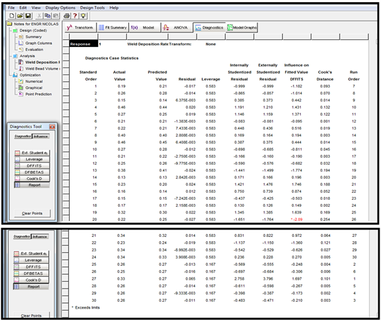
Figure 17. Diagnostics case statistics report of observed versus predicted weld deposition rate (WDR).

Figure 18. Reliability plot of observed versus predicted weld deposition rate (WDR).

Figure 19. Normal probability plot of studentized residuals for maximizing weld deposition rate (WDR).
residuals which is the number of standard deviation of actual values based on the predicted values was employed to ascertain if the residuals (observed-predicted) follows a normal distribution. It is the most significant assumption for checking the sufficiency of a statistical model. Result of Figure 19 revealed that the computed residuals are approximately normally distributed an indication that the model developed is satisfactory.
To determine the presence of a possible outlier in the experimental data, the cook’s distance plot was generated for the different responses. The cook’s distance is a measure of how much the regression would change if the outlier is omitted from the analysis. A point that has a very high distance value relative to the other points may be an outlier and should be investigated. The generated cook’s distance for deposition rate is presented in Figure 20.
The cook’s distance plot has an upper bound of 1.00 and a lower bound of 0.00. Experimental values smaller than the lower bound or greater than the upper bounds are considered as outliers and must be properly investigated. Results of Figure 20 indicates that the data used for this analysis are devoid of possible outliers thus revealing the adequacy of the experimental data.
To study the effects of current and voltage on deposition rate, 3D surface plots presented in Figure 21. To study the effects of gas flow rate and welding speed on deposition rate, 3D surface plots presented in Figure 22. The 3D surface plot as observed in Figure 22 and Figure 23, shows the relationship between the input variables (current and voltage), (welding speed and gas flow rate) against the response variables (weld deposition rate) It is a 3 dimensional surface plot which was employed to give a clearer concept of the response surface. Although not as useful as the contour plot for establishing responses values and coordinates, this view may provide a clearer picture of the surface. As the colour of the curved surface gets darker, the weld deposition rate increases proportionately. The presence of a coloured hole at the middle of the upper surface gave a clue that more points lightly shaded for easier identification fell below the surface.
Finally, numerical optimization was performed to ascertain the desirability of the overall model. In the numerical optimization phase, we ask design expert to maximize the weld deposition rate (WDR). In addition, the optimum current, voltage, welding speed and gas flow rate was determined simultaneously.

Figure 20. Generated cook’s distance for weld deposition rate (WDR).

Figure 21. Effect of current and voltage on weld deposition rate.

Figure 22. Effect of welding speed and gas flow rate on weld deposition rate.

Figure 23. Interphase of numerical optimization model for maximizing weld deposition rate (WDR).
The interphase of the numerical optimization of deposition rate showing the objective function is presented in Figure 23.
The constraint set for the numerical optimization algorithm is presented in Figure 24.

Figure 24. Constraints for numerical optimization of selected responses.
The numerical optimization produces about twenty two (22) optimal solutions which are presented in Figure 25.
From the results of Figure 25, it was observed that a current of 160.020 amp, voltage of 20.00 vol, a welding speed of 47.460 cm/min and gas flow rate of 17.000 L/min will result in a welding process with the following properties: Weld deposition rate (WDR) 0.436708 kg/hr. This solution was selected by design expert as the optimal solution with a desirability value of 98.80%.
The ramp solution which is the graphical presentation of the optimal solution is presented in Figure 26.
The desirability bar graph which shows the accuracy with which the model is able to predict the values of the selected input variables and the corresponding responses is shown in Figure 27.
It can be deduce from the result of Figure 27 that the model developed based on response surface methodology and optimized using numerical optimization method, predicted the weld deposition rate by an accuracy level of 99.39%. Finally, based on the optimal solution, the contour plots showing each response variable against the optimized value of the input variable is presented in Figure 28 and Figure 30. To identify the region with the optimum current and voltage, predicting the optimum deposition rate response a contour plot is produced in Figure 28.
To identify the region with the optimum gas flow rate and welding speed, predicting the optimum deposition rate response using contour plot is produced in Figure 29. To predict the desirability of the model a contour plot is produced in Figure 30.
As presented in Figures the contour plot can be employed to predict the optimum values of the input variables based on the flagged response variables.
3.2. Discussion
In this study, the optimization of weld deposition rate (WDR) was done using response surface methodology (RSM).The target of the optimization model was to Maximize the weld deposition rate, statistical design of experiment (DOE), using the central composite design method (CCD) was done. The design and optimization was executed with the aid of Design Expert 7.01.

Figure 25. Optimal solutions of numerical optimization model.

Figure 26. Ramp solution of numerical optimization.

Figure 27. Prediction accuracy of numerical optimization.
The model summary, which is presented as shown in Figure 5, revealed that the model is of the quadratic type, which requires the polynomial analysis order as depicted by a typical response surface design. To validate the suitability of the quadratic model the sequential model sum of squares were calculated for the response presented in Figure 6. To test how well the quadratic model can explain the underlying variation associated with the experimental data, the lack of fit test statistic was estimated for each of the responses.
The summary statistics of model fit shows the standard deviation, the r-squared and adjusted r-squared, predicted r-squared and the PRESS statistic for each complete model. Low standard deviation, R-Squared near unity and relatively low PRESS are the optimum criteria for defining the best model

Figure 28. Contour plot for optimum current.

Figure 29. Predicting weld deposition and voltage predicting the deposition raterate using contour plot.
source. Variance inflation factor (VIF) of approximately 1.0 as observed in Figure 7 was good since ideal VIF is 1.0. VIF’s above 10 are cause for alarm.
To understand the influence of the individual design points on the model’s predicted value, the model leverages were computed as presented in Figure 11. Leverage of a point varies from 0 to 1 and indicates how much an individual design point influences the model’s predicted values. A leverage of 1 means the predicted value at that particular case will exactly equal the observed value of the

Figure 30. Predicting desirability using contour plot.
experiment, i.e., the residual will be 0. Leverages of 0.6698 and 0.6073 calculated for both the factorial and axial points coupled with 0.1663 for the center point as observed in Figure 11 shows that the predicted values are close to the experimental values. Hence, lower residual value which shows the adequacy of the model.
In assessing the strength of the quadratic model towards maximizing the weld deposition rate (WDR), one way analysis of variance (ANOVA) figure was generated for deposition rate and result obtained is presented in Figure 12. To validate the adequacy of the quadratic model based on its ability to maximize the weld deposition rate (WDR) the goodness of fit statistics presented in Figure 13. From the result of Figure 13, it was observed that the “Predicted R-Squared” value of 0.8358 is in reasonable agreement with the “Adj R-Squared” value of 0.9108. Adequate precision measures the signal to noise ratio. A ratio greater than 4 is desirable. The computaed ratio of 17.704 as observed in Figure 13 indicates an adequate signal. This model can be used to navigate the design space and adequately maximize the weld deposition rate (WDR).
The optimal equation which shows the individual effects and combine interactions of the selected input variables (current, voltage, welding speed and gas flow rate) against weld deposition rate is presented based on actual factors in Figure 16 and Figure 17. The diagnostics case statistics which shows the observed values of (weld deposition rate (WDR) against their predicted values is presented in Figure 17. The diagnostic case statistics actually give insight into the model strength and the adequacy of the optimal second order polynomial equation, Lower residual values resulting to higher leverages as observed in Figure 17 is indicators of a well fitted model. To assess the accuracy of prediction and established the suitability of response surface methodology using the quadratic model, a reliability plot of the observed and predicted values of weld deposition rate is presented in Figure 18.
To determine the presence of a possible outlier in the experimental data, the cook’s distance plot was generated for the different responses. The Cook’s distance is a measure of how much the regression would change, if the outlier is omitted from the analysis. A point that has a very high distance value relative to the other points may be an outlier and should be investigated. The generated cook’s distance for deposition rate is presented in Figure 20. To study the effects of current and voltage on deposition rate, 3D surface plots presented in Figure 22.
The 3D surface plot as observed in Figure 22 and Figure 23, shows the relationship between the input variables (current and voltage), (welding speed and gas flow rate) against the response variable (weld deposition rate). It is a 3 dimensional surface plot, which was employed to give a clearer concept of the response surface. Although not as useful as the contour plot for establishing responses values and coordinates, this view may provide a clearer picture of the surface. As the colour of the curved surface gets darker, the weld deposition rate and the weld bead volume increase proportionately. The presence of a coloured hole at the middle of the upper surface gave a clue that more points lightly shaded for easier identification fell below the surface.
Finally, numerical optimization was performed to ascertain the desirability of the overall model.
From the result of Figure 25, it was observed that a current of 160.020 amp, voltage of 20.00 vol, a welding speed of 47.460 cm/min and gas flow rate of 17.000 L/min will result in a welding process with weld deposition rate (WDR) 0.436708 kg/hr. This solution was selected by design expert as the optimal solution with a desirability value of 98.80%.
The desirability bar graph, which shows the accuracy with which the model is able to predict the values of the selected input variables and the corresponding responses, is shown in Figure 18. It can be deduced from the result of Figure 27 that the model developed, based on response surface methodology and optimized, using numerical optimization method, predicted the weld deposition rate by an accuracy level of 99.39%. Finally, based on the optimal solution, the contour plots showing each response variable against the optimized value of the input variable are presented in Figure 28 and Figure 29, respectively. To identify the region with the optimum current and voltage, predicting the optimum deposition rate response a contour plot is produced in Figure 28. To identify the region with the optimum gas flow rate and welding speed, predicting the optimum deposition rate response, a contour plot is produced in Figure 29.
4. Conclusion
In this study, the response surface methodology to optimize the deposition rate of TIG welded joints and result shows that they are suitable models. Weld deposition rate is a very important factor that influences the integrity and quality of welded joint. The study reveals that respond surface methodology (RSM) produced a good model for predicting weld deposition rate. it was observed that a current of 160.020 amp, voltage of 20.00 vol, a welding speed of 47.460 cm/min and gas flow rate of 17.000 L/min will result in a welding process with weld deposition rate (WDR) 0.436708 kg/hr. It has been shown that the optimization and prediction of weld deposition rate has improved the quality of welded joints. A weld simulation was carried out using the optimum value obtained from the response surface methodology to produce a welded sample with good quality. It is, therefore, recommended that welding and fabrication industries should endeavor to use the optimum welding process parameters obtained in this study to produce high quality welds in Tungsten inert gas welding process, as applicable.
Conflicts of Interest
The authors declare no conflicts of interest regarding the publication of this paper.
Cite this paper
Imhansoloeva, N.A., Achebo, J.I., Obahiagbon, K., Osarenmwinda, J.O. and Etin-Osa, C.E. (2018) Optimization of the Deposition Rate of Tungsten Inert Gas Mild Steel Using Response Surface Methodology. Engineering, 10, 784-804. https://doi.org/10.4236/eng.2018.1011055
References
- 1. Nand, S. and Singh, P.K. (2015) Effect of Addition of Metal Powder on Deposition Rate, Mechanical Properties, and Metallographic Property of Weld Joints during Submerged Arc Welding Process. Journal of Machining and Forming Technologies, 6, 3-4.
- 2. Clark, D., Bache, M.R. and Whittaker, M.T. (2008) Shaped Metal Deposition of a Nickel Alloy for Aero Engine Applications. Journal of Materials Processing Technology, 203, 439-448. https://doi.org/10.1016/j.jmatprotec.2007.10.051
- 3. Benyounis, K.Y., Olabi, A.G. and Hashmi, M.S.J. (2008) Multi-Response Optimization of CO2 Laser Welding Process of Austenitic Stainless Steel. Optics & Laser Technology, 40, 76-87. https://doi.org/10.1016/j.optlastec.2007.03.009
- 4. Hooda, A., Dhingra, A. and Sharma, S. (2012) Optimization of Mig Welding Process Parameters to Predict Maximum Yield strength in Aisi 1040. IJMERR, 1, 203-213.
- 5. Juang, S.C. and Tarng, Y.S. (2002) Process Parameters Selection for Optimizing the Weld Pool Geometry in the Tungsten Inert Gas Welding of Stainless Steel. Journal of Materials Processing Technology, 122, 33-37. https://doi.org/10.1016/S0924-0136(02)00021-3
- 6. Choi, J. and Chang, Y. (2005) Characteristics of Laser Aided Direct Metal/Material Deposition Process for Tool Steel. International Journal of Machine Tools and Manufacture, 45, 597-607. https://doi.org/10.1016/j.ijmachtools.2004.08.014
- 7. Singh, V. (2013) An Investigation for Gas Metal Arc Welding Optimum Parameters of Mild Steel AISI 1016 Using Taguchis Method. International Journal of Engineering and Advanced Technology (IJEAT), 2, 407-409.
- 8. Thakur, P.P. and Chapgaon, A.N. (2016) A Review on Effects of GTAW Process Parameters on Weld. International Journal for Research in Applied Science & Engineering Technology (IJRASET), 4, 136-140.
- 9. Achebo, J.I. (2011) Optimization of GMAW Protocols and Parameters for Improving Weld Strength Quality Applying the Taguchi Method. Proceeding of the World Congress on Engineering, Vol. 1, WCE 2011, London, 6-8 July 2011.
- 10. Schneider, C.F., Lisboa, C.P., Silva, R.A. and Lermen, R.T. (2017) Optimizing the Parameters of TIG-MIG/MAG Hybrid Welding on the Geometry of Bead Welding Using the Taguchi Method. Journal of Manufacturing and Material Processing, 1, 14. https://doi.org/10.3390/jmmp1020014