Open Journal of Modelling and Simulation
Vol.03 No.04(2015), Article ID:60456,31 pages
10.4236/ojmsi.2015.34017
Multiple Levels of Abstraction in the Simulation of Microthreaded Many-Core Architectures
Irfan Uddin
Institute of Information Technology, Kohat University of Science and Technology, Kohat, Pakistan
Email: mirfanud@kust.edu.pk
Copyright © 2015 by author and Scientific Research Publishing Inc.
This work is licensed under the Creative Commons Attribution International License (CC BY).
http://creativecommons.org/licenses/by/4.0/


Received 14 September 2015; accepted 19 October 2015; published 22 October 2015
ABSTRACT
Simulators are generally used during the design of computer architectures. Typically, different simulators with different levels of complexity, speed and accuracy are used. However, for early design space exploration, simulators with less complexity, high simulation speed and reasonable accuracy are desired. It is also required that these simulators have a short development time and that changes in the design require less effort in the implementation in order to perform experiments and see the effects of changes in the design. These simulators are termed high-level simulators in the context of computer architecture. In this paper, we present multiple levels of abstractions in a high-level simulation of a general-purpose many-core system, where the objective of every level is to improve the accuracy in simulation without significantly affecting the complexity and simulation speed.
Keywords:
High-Level Simulations, Multiple Levels of Abstraction, Design Space Exploration, Many-Core Systems

1. Introduction
With the current trend of many-core systems, we interpret Moore’s law as the number of cores will be doubled every new generation of processor. We believe that in the near future we will have more than a thousand cores on a single die of silicon and therefore the use of high-level simulators in the design of such complex systems cannot be avoided. Using space sharing, as well as time sharing, the mapping of applications onto such systems can be very complex. Any decision to improve the performance of the architecture becomes expensive at the later stages of design and requires more effort, time and budget. Therefore, simulators with high simulation speed and less complexity are desirable for efficient Design Space Exploration (DSE) of the architecture. Computer architects need to perform DSE before the design is printed onto silicon and even after manufacturing to optimise the performance of the architecture for critical applications.
DSE is performed in all kinds of computer systems. However, in the embedded systems domain, the use of high-level simulation for DSE purposes has been accepted as an efficient approach for more than a decade [1] . In that sense, DSE in embedded systems has pioneered high-level simulation techniques. Embedded systems perform predefined tasks and therefore have particular design requirements. They are constrained in terms of performance, power, size of the chip, memory etc. They generally address mass products and often run on batteries, and therefore need to be cheap to be realized in silicon and power efficient. Modern embedded systems, typically have a heterogeneous Multi Processor-System-on-Chip (MP-SoC) architecture, where a component can be a fully programmable processor for general-purpose application or a fully dedicated hardware for time critical applications. This heterogeneity makes embedded systems more complex and therefore designers use high-level simulator to perform DSE at an early stage because of the short development times.
We want to clearly distinguish between application-dependent DSE in traditional embedded systems and application-independent DSE in modern embedded systems or generalpurpose computers. In traditional embedded systems, applications are statically mapped to different configurations of an architecture using a pre-defined mapping function. Based on simulation results, innovative ideas can be generated which can improve application, mapping strategies and architecture separately, be it for power or performance. However, in modern embedded systems there is not one particular application or scenario, but a range of applications targeted to different configurations of the architecture. For instance in smart phones the range of applications is similar to a general purpose system and hence there are many types of application that must be mapped together with the critical functions of the device. In this way, modern embedded systems are converging towards general-purpose systems. In these situations, the mapping of an application cannot be analyzed statically and in isolation but instead the code patterns in algorithms are analyzed, and dynamic mapping is used where different processes in an application are mapped to the architecture based on certain objectives. Because of the dynamic mapping, application-independent DSE is not as trivial as scenario-based DSE.
The growing number of cores and size of the on-chip memory are now beginning to create significant challenges for evaluating the design space of future general-purpose computers. We need scalable and fast simulators for the exploration of the design of these systems if this is to be achieved in a limited development time and budget. Commercially available processors in the market today have few cores on a chip e.g. Intel E708800 Series, IBM’s POWER7 and AMD’s Opteron 600 Series. In the near future we believe commercial processors will have hundreds of cores per chip and DSE at the early stage can no longer be avoided [2] . In special-purpose domains this number may even be in the thousands. The use of high-level simulators for DSE in general-purpose computers is relatively new compared to the embedded systems domain. A number of high-level simulation techniques are being developed as high-speed simulators for the DSE in general-purpose computers is relatively new compared to the embedded systems domain. A number of highlevel simulation techniques are being developed as high-speed simulators for the DSE in generalpurpose computers (c.f. Section 8). These have less complexity and a shorter development time when compared to detailed cycle-accurate simulators. The techniques used are diverse and do not follow a particular pattern as in the case of DSE for embedded systems.
In the early stages, the time to produce results for the verification of a design for an architecture is critical and therefore short development time is also desirable in simulators. In DSE a huge design space is required to be explored and therefore high simulation speed cannot be avoided. A cycle-accurate simulator simulates all the low-level details of the architecture and therefore a large number of parameters are required to be considered in the exploration process which results into combinatoric explosion when choosing parameters with different combinations in order to change the configuration of the architecture. Therefore we need to abstract these low-level details to provide an abstracted simulator. Accuracy is desirable, but it is not possible to achieve the highest possible accuracy in abstracted simulations.
In this paper we propose multiple levels of high-level simulation techniques for general-purpose, many-core systems and address the challenge of finding a level that takes less development time, provides reduced complexity, achieves high simulation speed and exhibits reasonable accuracy. This research challenge is illustrated in Figure 1. RTL models or cycle-accurate models are accurate, but they are complex, slow and take a considerable amount of time in development. They consider all design points and therefore suffer from combinatoric
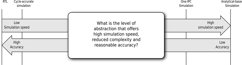
Figure 1. The research challenge in the simulation of many-core systems.
explosion when used in DSE. On the other side we have analytical models which are fast and least complex but do not consider the adaptation based on the dynamic state of the system and resource sharing. There are one IPC (Instruction per cycle) based simulation techniques which are less complex, fast but are not accurate.
We are proposing the high-level simulation techniques by considering a particular implementation of the microthreading model [3] known as the microthreaded, many-core architecture also termed the Microgrid [4] . Since the Microgrid is a complex architecture, we need high-level simulators to perform DSE. These simulation techniques are also applicable to current and future many-core systems such as Intel SCC, TILE64, Sun/Solaris Tx etc., with modifications to the architectural parameters. The contribution of this research is the introduction of multiple levels of the high-level simulation techniques and the engineering of the framework for early design space exploration of the Microgrid that aims for short development time, reduced complexity, faster simulation speed with the cost of losing some accuracy.
The rest of the paper is organized as follows. We give background of the microthreaded many-core systems i.e. Microgrid in Section 2 and then describe why simulation is desired during the design of an architecture particularly many-core systems in Section 3. We give multiple levels of abstractions generally used in the simulation of computer architecture in Section 4. In Section 5, we give an overview of the multiple levels of the simulation technique for the microthreaded many-core systems. The framework of the high-level simulator for the Microgrid is explained in Section 6 and the results achieved from the simulation framework for the Microgrid in Section 7. We describe the related work in Section 8, an overview of the lessons we have learned from this research in Section 9 and the conclusion of the paper in Section 10.
2. Background
The Microgrid [5] is a general-purpose, many-core architecture which implements hardware multi-threading using data flow scheduling and a concurrency management protocol in hardware to create and synchronize threads within and across the cores on chip. The suggested concurrent programming model for this chip is based on fork-join constructs, where each created thread can define further concurrency hierarchically. This model is called the microthreading model and is also applicable to current multi-core architectures using a library of the concurrency constructs called svp-ptl [6] built on top of pthreads. In our work, we focus on a specific implementation of the microthreaded architecture where each core contains a single issue, in-order RISC pipeline with an ISA similar to DEC/Alpha, and all cores are connected to an on-chip distributed memory network [7] . Each core implements the concurrency constructs in its instruction set and is able to support hundreds of threads and their contexts, called microthreads and tens of families (i.e. ordered collections of identical microthreads) simultaneously. This implementation is referred as the Microgrid. In the rest of the paper a thread means a microthread, and a core means microthreaded core unless stated otherwise. An example layout of the 128-core Microgrid in a single chip is shown in Figure 2.
To program this architecture, we use a system-level language called SL [8] which integrates the concurrency constructs of the microthreading model as language primitives. We show an example program i.e. Matrix Multiplication of equal sized matrices, to demonstrate the way programs are written for the Microgrid. The objective is to show that a sequential C program can be transformed to a microthreaded program easily by high-level programming languages, a compiler or with little effort by the programmer. We also show the concurrency constructs in the SL program to demonstrate the concurrency management on the Microgrid.

Figure 2. The layout of 128 cores on the microgrid chip.
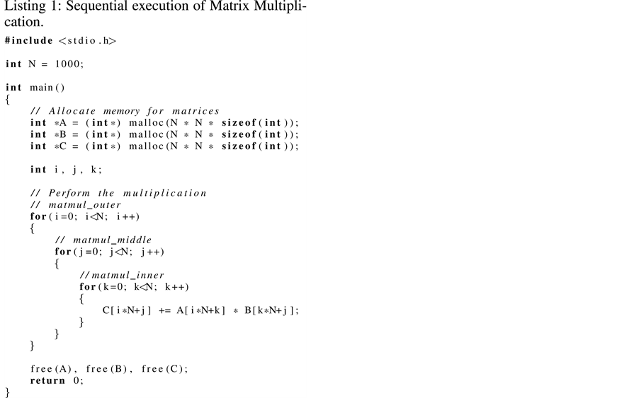
The sequential C code for Matrix Multiplication of size 1000 × 1000 is shown in Listing 1. We allocate three arrays; two for source matrices and one for the result matrix. Once the memory is allocated, we would normally fill these arrays with numbers, but to save space on the page, we assume the existing values present in those memory locations. To perform matrix multiplication we write three loops: the outer loop, middle loop and inner loop. The inner loop is the one which performs the inner product of the two vectors of the source matrices identified by the outer loops and stores in the scaler result in the result matrix. After the matrix multiplication is completed, we free the allocated memory.
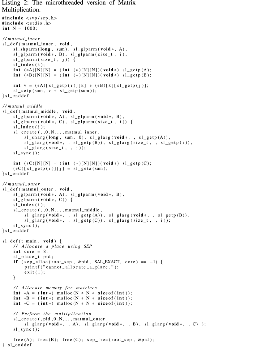
The microthreaded program for the Matrix Multiplication of size 1000 × 1000 written in SL is shown in Listing 2. The statements with prefix sl_ are SL constructs and used for the concurrency management in the Microgrid. In the t_main function, we first allocate a group of 8 cores in the Microgrid called a place and identified by the place identifier pid. Then we allocate three arrays for source and result matrices. Then we replace the outer loop by creating a family of N threads. The threads in the outer family create further middle families and then each of those creates the inner family. The inner family performs the inner product as a sequential reduction described as concurrent threads, with dependencies between threads. This allows the multiplications to be performed concurrently but constraining the sum to be performed sequentially. Thus the SL program captures all concurrency available in the algorithm but any implementation of it will necessarily schedule this according to
resources available, i.e. cores, families, threads etc. The transformation from sequential program to microthreaded program involves the creation of families with shared and global parameters. Global parameters are read only in a thread and carry constants like the addresses of the arrays. Shared parameters are write once in a thread and are read by the subsequent thread in a family and are used here to constrain the inner threads to perform the reduction sequentially. Once all the families are synchronized, the allocated memory to arrays and allocated cores are released.
It should be noted that some components typically associated with the kernel of an operating system are subsumed by the SL language and its constructs and, in the Microgrid, implemented in the core’s ISA. For example sl_create maps directly to a create instruction in the assembly code, which together with other supporting instructions schedules the concurrency defined in the code onto the available resources as allocated and identified by the place identifier pid. This in turn has implication in the implementation of OS services on the Microgrid. The SL system for the Microgrid supports a range of OS services with familiar encapsulation making migration from existing systems relatively simple.
MGSim is the cycle-accurate simulation framework [9] -[11] and HLSim is the high-level simulation framework [12] [13] of the Microgrid. HLSim is developed to make quick and reasonably accurate design decisions in the evaluation of the microthreaded architecture using multiple runs of benchmarks which may comprise the execution of billions of instructions. It also allows us to investigate mapping strategies of families to different numbers of cores in developing an operating environment for the Microgrid. The high-level simulator provides us a simple way to model the microthreaded cores in large-scale system, avoiding all the details of executing instruction streams of a thread and to focus more on mapping, scheduling and communication of threads and families. The high-level simulation is not meant to replace the cycle-accurate simulation, rather complementing it with some techniques that are fast enough to explore the architecture more widely. We think of the high-level simulation as a useful tool in the designer’s toolbox for design space exploration, which is faster and less complicated in simulating the architecture. As this paper explains, we have multiple levels of HLSim where the objective of each level is to keep the simulation technique simple and increase the accuracy without affecting the simulation speed. These different levels are explained in Section 5.
Simulators are tools to reproduce abstract models of components behaviors in order to make predictions. These are useful tools in the designer’s toolbox to explore the behavior of components before the design is finalized. Emulators on the other hand are tools to reproduce the concrete behavior of a computing artifact, i.e. the hardware and software interface of a given processor. These tools are generally used during compiler and oper-
ating systems development to debug software in a controlled environment before it ships to production. These definitions are based on the explanation given in [14] . In summary, simulators exist to debug and optimize hardware designs, whereas emulators can be further divided between partial and full system emulators. Partial emulation only executes application within emulation environment and operating software functions are serviced through the host machine. With a full emulation, the entire software stack runs on the emulated hardware. This paper is all about simulation (multiple levels of HLSim), however for the verification we use a full-system emulator implemented by MGSim, the cycle-accurate simulation of a Microgrid.
In the simulation of computer architecture there are two important phases; specification and modelling. The specification of an architecture is that when the simulation is used to predict behavior and guide design, but where verification is not possible. The focus of MGSim is specification. The modelling phase is used to simplify complexity and validation is available to quantify accuracy. The focus of HLSim is modelling.
3. Simulation of Computer Systems
Modern processors integrate billions of transistors on a single chip, implement multiple cores along with on-chip peripherals and are complex pieces of engineering. In addition, modern software is increasingly complex and includes commercial operating systems on virtual machine with an entire application stack. Computer architects need simulators for the evaluation of the architecture for obvious reasons, like complexity in the design, development/manufacturing time, effort and cost of changing the configuration of components in the silicon etc. The complexity in the architecture and software makes the simulation of the modern computer system more challenging. The problem is further exacerbated in many-core or System-on-Chip (SoC) designs where a large number of components results in a huge design space to be explored.
Simulations are essential in the overall design activity of computer architecture and are used at different levels of details shown in Figure 3 (Originally presented in [15] but here we have slightly modified it). Each level has a different level of simulation speed, development time, complexity and accuracy. The width of the pyramid indicates the number of design points at each stage, at the top the width is very small as the low-level details are not available but as we go towards the bottom the design space increases because of the increased number of low-level specifications. The parameters affecting the design of an architecture are shown on the sides of the pyramid, and they change on going from bottom to top and vice versa. Therefore, there is always a trade-off between these parameters when simulating an architecture at a given level.
Simulation in computer architecture is an iterative process. Practitioners go from top to bottom, and then bottom to top again. These iterations are necessary, because the top to bottom approach often fails to detect that some high-level ideas cannot be implemented because of conceptual errors, technology errors etc. Only when the low-level approaches have been tried, the practitioners understand the problems better and therefore the

Figure 3. The design pyramid used in the design process of computer architecture.
high-level approaches need to be adapted (or re-implemented).
Pen and paper models: The pen and paper model is generally the first step in the computer architecture design. A prototype architecture can be designed with enough experience in the domain of computer architecture. The computer architects/designers have knowledge and intuition about the components that can be used in order to achieve efficiency and can predict the performance of the system. Based on certain assumptions and estimations the designer can draw the overall layout of the architecture.
Analytical models: Analytical models, e.g. [16] , are generally used after pen and paper models to validate the model mathematically. They generally involve some simple spreadsheets or some mathematical validation of the design. In the design pyramid going from top to bottom we validate the model, but going from bottom to top the architecture can be explored using empirical data. While the former approach is already explored for the Microgrid in [16] , we have explored the later approach in [17] .
System-level/High-level models: System-level or High-level models are relatively new in the simulation of general-purpose computers [18] . These models are meant to provide a reduced complexity in simulation which requires less development effort and provide high simulation speed with the cost of loosing some accuracy. These simulators are abstract, and therefore are good candidates for design space exploration of the architecture. Although this model comes after analytical models time wise, they are typically exploited only after cycle- accurate models have been developed. Computer architects generally start from the bottom, after pen and paper models. This is an engineering approach and is commonly used. The progression down the design pyramid is an ideal situation that is rarely seen in practice.
Cycle-accurate models: The design of the architecture stays fluid through simulation in order to realize a validated system in silicon and to provide further optimizations in the silicon chip. The most commonly used simulation technique in academia and industry is the detailed, event-driven simulation of all the components of the architecture [7] [19] . Detailed simulation is generally the first step in the design process of an architecture soon after pen and paper model and analytical models. These simulators are complex, take considerable effort in development, execute slowly on contemporary hardware but above all provide accurate results. SimpleSCalar [20] , COTSon [21] , SimOS [22] , Simics [23] etc. are some examples of the cycle-accurate simulators.
RTL models: RTL (Register Transfer Level) or VHDL (Verilog Hardware Description Language) models are used to describe the way components are connected on the chip to execute the code, this may be at the gate level. These models are written in software, can be simulated and can subsequently be synthesized to generate the silicon chip or FPGA prototype. The writing of VHDL code is complex and requires more development effort than cycle-accurate simulators.
Hardware: The ultimate goal of computer architects is to realize the design of the architecture in silicon, which is complex engineering work and requires even more effort and budget. The alternative approach to a silicon chip is the FPGA prototype [24] with relatively small engineering effort and budget. Silicon chips and FPGA prototypes give the highest execution speed and accuracy but have the largest design space to be explored because of the large number of low-level parameters.
4. Raising the Level of Abstraction in the Simulation
Cycle-accurate simulation for the evaluation of a computer architecture is a mature technology. With a considerable amount of development effort these complex pieces of software can be engineered. They implement all the components of the system in detail and therefore provides the highest possible accuracy of the simulated hardware in software. However, in early system-level design, decisions related to e.g. performance, power, network type etc., the highest accuracy is not always desirable and therefore using a detailed simulator is not justifiable.
A set of benchmarks which may contain billions of dynamically executed instructions are used for the evaluation of an architecture. The execution of such a large number of instructions in a cycle-accurate simulator will take a huge amount of wall clock time which will be many orders of magnitude higher than the time taken by the real processor to execute the benchmarks. In order to determine the successful future of an architecture design, evaluation of a variety of system parameters in a short amount of time is critical and therefore cycle-accurate simulation is not very useful. The problem is further exacerbated in many-core systems as software components can be space-shared in many different configurations. In fact the greater the number of cores, the greater the combinatoric explosion in the number of configurations that need to be explored.
Cycle-accurate simulations are generally single-threaded as a multi-threaded implementation will result in a large number of synchronization points between the simulated cores and will affect the simulation time significantly. If we have a loosely dependent systems (e.g. distributed systems on chip), then multi-threading can provide benefits in faster execution. With the current trend in technology of contemporary hardware the number of cores on a single chip is increasing and the frequency of the single core or hardware thread is decreasing. Therefore cycle-accurate simulators will execute more slowly on future multi-cores machines than on the current multi-cores. Although the number of instances of the simulator that can be started on different cores of the host machine can be increased and this technique can be used to explore different parameter combinations. However, simulating large single applications will still take more simulation time.
Keeping in mind the modern interpretation of Moore’s law, the cost of development and execution in simulating a large number of cores in cycle-accurate simulators is becoming increasingly expensive. With the number of cores in a system scaling up to hundreds or thousands, we believe that the IPC (Instruction Per Cycle) of a single core becomes less interesting to simulate. Instead of modelling the performance of individual cores, the focus of simulation needs to shift towards the overall behavior of the chip, where the creation, communication and synchronization of concurrency plays a central role.
Clearly there is a need to raise the level of abstraction from detailed simulation to high-level simulation. Faster execution is not the only objective, the other objectives are a shorter development time, reduced complexity while maintaining a reasonable accuracy. An abstracted simulator can be used to determine a particular configuration (be it application, architecture or both) that gives the best result (be it performance or power) across a range of applications. For instance, in investigating the size of the thread table, if increasing the size of the thread table after a particular size does not affect the performance across a range of applications, then the hardware budget and or energy budget can be reduced. These experiments can be performed using either a cycle- accurate simulator or a high-level simulator. But the high-level simulator can more quickly perform the design space exploration to determine that particular thread table size. This design change can then be implemented in the cycle-accurate simulator. In this way we can save a lot of time in executing an application for different configurations of the thread table size in the cycle-accurate simulator. Further a particular area of interest in the architecture or application, determined by the high-level simulator can be further analyzed in detail using the cycle-accurate simulator.
On the other hand, cycle-accurate simulators are required in order to validate the design, as without the detailed simulation the designers have no idea whether the design of the architecture is correct and can achieve the same results as expected. Furthermore, high-level simulation needs to be calibrated, verified and validated which is not possible without the detailed simulation, FPGA prototype or silicon chip. In the absence of silicon chip or fully developed FPGA prototype, the need of the cycle-accurate simulation cannot be avoided. Even if the silicon chip is available, a cycle-accurate simulator is used because it is easier to change the configuration of the design and it provides greater flexibility in investigating potential problems, such as deadlock.
High-level simulation is a relatively new topic of research in the simulation of general-purpose many-core architecture. As the transition from system-level model to RTL model [18] is not straightforward, system-level simulation is considered as an extra effort and has never become a mature technology. But with the current trend in many-core systems, DSE in general-purpose computers cannot be avoided and hence high-level simulators become a necessity. Computer architects always strive to have the most efficient architecture, and therefore keep exploring the architecture with different configurations throughout the design and also after the realization of the design in silicon. Therefore we believe that high-level simulators in the future will be commonly used for DSE in general-purpose many-core systems.
5. Multiple Levels of Abstraction
A number of implementations are available for the evaluation of the Microgrid, as shown in Figure 4. There are researchers working in UTIA on UTLEON [7] [19] to develop an FPGA prototype of the Microgrid. At the time of writing only a single core of the Microgrid has been simulated in FPGA. However, it provides faster execution and could provide the same accuracy as silicon chip but it was complex to design and requires modification to become a cycle accurate simulation of a custom chip. There are also limited opportunities to implement changes in the prototype after making changes in the design due to implementation constraints. There are researchers working in the CSA group on MGSim [24] to provide a detailed simulation of the Microgrid. The detailed simulation is accurate and more flexible that the FPGA but very slow in execution, complex and takes a

Figure 4. Multiple levels of simulation for the microgrid, and multiple levels in the high-level simulation of the microgrid.
lot of development effort (c.f. Section 7). The focus of the research work presented in this paper is to provide multiple levels of abstraction in the high-level simulation of the Microgrid, to achieve a high simulation speed, reduced complexity, short development time with a compromise on the accuracy.
In HLSim we propose multiple levels of abstraction where a level can be used based on the trade-off amongst complexity, simulation speed and accuracy. In design space exploration high simulation speed and less complexity is desired. We only need relative accuracy or fidelity in high-level simulation. However, in order to increase the accuracy we need to simulate further components of the architecture which affects the simulation speed. In the multiple levels of HLSim, we have tried to improve the accuracy without affecting the simulation speed and complexity. We give an overview of these different levels below.
・ Front-end HLSim: It simulates the application model of the simulation framework without any integration with the architecture model. It provides a run-time system for the execution of microthreaded programs on any host machine. This model is explained in [6] .
・ One-IPC HLSim: It simulates the architecture model of the simulation framework. As the Microgrid provides fine-grained latency tolerance, it is likely that the throughput of the program can achieve an execution rate of one instruction per cycle on a single-issue core. We are using this assumption to develop the architecture model. This level completes the framework of the high-level simulation to perform performance- aware DSE. The simulation framework is explained in [12] [13] [25] .
・ Signature-based HLSim: This level introduces a basic block analyzer to estimate the numbers of different classes of instructions in the basic block of microthreaded program, which is stored in signature for that block. The signature is a high-level categorization of low-level instructions. Signatures are then used to estimate the performance of the basic block based on the number of instructions, type of instruction and the number of active threads in the pipeline. This model is presented in [26] [27] .
・ Cache-based HLSim: The Signature-based HLSim was an attempt to improve the accuracy of simulation by dynamic adaptation of the throughput based on the state of the system (number of active threads). However, it does not consider the access time of load or store operations to different levels of the cache, these form a single class in Signature-based HLSim. Accessing different levels of the memory system have different latencies and hence in Cache-based HLSim we add an intelligent estimation of the cache hit rates to the basic blocks in Signature-based HLSim in order to consider the access to different levels of the cache in the distributed memory network on the chip. This simulation technique is presented in [28] .
・ Analytical-based HLSim: The above simulation techniques are still based on abstracted instruction execution, as every concurrency event is required to be accounted for and simulated on the host machine. Given that the behavior of the application and the architecture is known, we can abstract the execution of a whole component by using an empirical estimate of its throughput from the cycle-accurate simulator, MGSim. In this level we achieve the highest possible simulation speed and reduced complexity. The Analytical-based HLSim is described in [17] .
The trade-off between accuracy and simulation speed is a complex one. The fastest simulation speeds are obtained using Analytical-based HLSim but this is based on the component being evaluated once in MGSim, stored and then used many times as a component within HLSim. This it is applicable to library components such as equation solvers, linear algebra functions, etc. Of the other techniques the accuracy is dependent on the application. For example an application that is compute bound would not merit the use of Cache-based HLSim, which again requires some prior analysis in MGSim. However, for memory bound applications significant improvements in accuracy and fidelity can be obtained for very little additional simulation time.
6. High-Level Simulation
6.1. Separation of Concerns
In the Microgrid design we have parameters to change the execution of the application on concurrent system, and we have parameters to change the configuration of the architecture. The programmer can choose different parameters, in order to achieve the best possible results, be it performance or power utilization. In the context of the Microgrid, application parameters are window size, cold/warm caches, place size etc. and the architecture parameters are thread table size, family table size, frequency of cores, network type, memory configuration etc.
・ Application parameters:
○ Application type: The high-level cache-model is an application-dependent model, and therefore it is impossible to derive a model to be used by different applications. Some applications will exploit locality, some will not, or indeed some applications may exhibit different characteristics at different stages of the application.
○ Input data type/size: The size of the input problem is known to have affect on the cache access patterns, but in some cases (e.g. sorting) the input data values can also affect the algorithm and hence the cache access pattern.
○ Window size: It is a run-time parameter and it limits the number of threads per family created on each core. The reason is to leave space for other threads in the application, for example to statically avoid deadlock. Different ratios of threads from different families running on a core can impact its performance, though efficiency and locality issues.
○ Place: The place is a handle to the set of hardware resources used to create a family of threads. It determine the number of cores and their concurrency resources (threads, families etc.), and the location of the cores on the chip.
○ Cold/Warm caches: If the data has not been loaded previously into cache it is called a cold cache and if the data already exists in the cache, then the cache is called warm. We need to consider both cases, as the access pattern in either case can be different and the high-level cache model presented in Cache-based HLSim needs to be aware of this.
・ Architecture parameters:
○ Size of L1-cache and L2-cache: The size of caches has an effect on the performance of the application.
○ Associativity of L1-cache and L2-cache: The associativity in caches can have an affect on the performance of the application.
○ Number of L1-caches sharing L2-cache: The number of L1-caches, sharing an L2-cache changes the access pattern of caches in the application.
○ Number of L2-caches in low-level ring network: The number of L2-caches in the low-level ring network affect the cache access pattern and the load of the messages on the low-level ring network.
○ Number of low-level rings in top-level ring: The number of low-level rings on the chip affect the flow of messages on the chip and out of the chip.
○ Frequency of core, caches and DDR: Frequency changes the access time of accessing a particular region on the chip.
○ Thread table size, family table size, register file size: These parameters affect the number of threads, families and how many registers can be allocated. The number of register can also affect the number of simultaneous threads to be allocated.
○ Synchronization-aware coherency protocol: The coherency protocol can change the load on the on-chip memory network.
○ Topology of the memory architecture: Although we are simulating ring topology in this paper, we are interested to simulate other topologies and protocols, and that has to be considered in the high-level cache model.
Because of the separate application and architecture parameters, we see a strict separation of concerns [29] between application model and the architecture model and either one can be improved from simulation results. For instance, changing the place parameter can change the performance achieved in the application, and changing the configuration of the number of caches in the ring can change the performance achieved on the architecture. In order to have separation in the application and architecture model, we can work independently on either model towards the overall performance. Because of this advantage, we have used separation of concerns during the design of HLSim. The separation of concerns is based on the famous Y-chart approach [15] shown in Figure 5. In the context of HLSim, the mapping layer does not exist explicitly because concurrency is decided at run-time and therefore can be improved implicitly with the improvement in the application.
6.2. HLSim Framework
The high-level simulation of the Microgrid is an implementation of a discrete-event simulation [30] . The simulation framework of HLSim is shown in Figure 6 and consists of three parts.
・ Application model: This is the microthreaded program that executes on the host machine, but generates events with the estimates for concurrency and abstract details of each block of instructions. It provides the fully functional execution of the microthreaded program on the host machine and there are parameters that can be changed that impact the simulation results through the architecture model below, e.g. place size, window size etc.
・ Mapping function: The events generated by the application model are stored in an ordered queue where the top of the queue represent the event with the least workload. This layer is responsible for passing timing information to the architecture model and can be changed implicitly with changes in the application model.

Figure 5. The Y-chart approach.

Figure 6. The simulation framework of HLSim. The application model provides the front-end to write microthreaded programs. The architecture model provides the back-end simulating the Microgrid at an abstract level. Mapping function maps events from the application model to the architecture model and the acknowledgement to the application model.
・ Architecture model: This layer simulates the hardware resources of the microthreaded, many-core architecture. It provides location of execution, simulated time, distribution of threads on cores etc. to the application model. We are using different types of the architecture model based on different abstractions of the hardware resources, i.e. One-IPC HLSim, Signature-based HLSim, Cache-based HLSim and Analytical- based HLSim.
The events for the concurrency constructs are blocking and computational blocks are non-blocking. By blocking we mean that the application model stops execution until notified by the architecture model, and by non-blocking we mean that the application model keeps sending events without any acknowledgement until the next blocking event is generated and blocked by the architecture model.
7. Evaluation
In this section we give the configuration of the host machine and the benchmarks we are using for an evaluation of the multiple levels of HLSim against the cycle-accurate simulator MGSim. As per the objectives of this research, we identify the development time and complexity of the different simulators. We also present results to show how accuracy improves as we simulate more and more details of the architectural resources in HLSim. We show results as absolute and relative accuracy for all levels of HLSim compared to MGSim. The important conclusion is that, under reasonable assumption in terms of use, the simulation speed is not significantly affected with the improved accuracy.
7.1. Configurations
In this section we give the configuration of the host machine, MGSim and HLSim.
Host machine: This is the platform where both simulators are executing. The model of the processor is Quad-Core AMD Opteron (tm) Processor 8356. It has 4 physical processors, each consisting of 4 physical cores (these are not microthreaded cores). In total we have 16 physical cores each running at 2.3 GHz. It has 64 KB L1 instruction and data cache. Every core has a private 512 KB L2-cache and every processor (i.e. 4 cores) has a 2048 KB L3-cache.
7.2. Development Effort
One of the issues raised in the introduction is the development effort in producing a simulator either from scratch or in some cases based on prior developments. Because of the unique features of the Microgrid, development of simulators was made from scratch. The exception to this is UTLEON, with was based on the LEON III open-source code. We therefore present estimates of development time based on the number of person months required for the different simulators. The aim was to demonstrate the relatively short development time of the high-level simulator compared to the cycle-accurate simulator and FPGA prototype. The person months are calculated based on the number of full-time PhDs required to complete each part of the project. One full- time PhD requires approximately 40 person months.
・ UTLEON: The estimated development time was 160 person months, and the objective was to develop an FPGA prototype for the single core of the Microgrid. In other words 4 full-time PhDs worked on this prototype.
・ MGSim: The estimated development time was 80 person months, and the objective was to write a detailed simulator for many-cores of the Microgrid. In other words two full-time PhDs were involved in the development.
・ HLSim: The estimated development time was 40 person months, and the objective was to write multiple levels of an abstract simulator for many-cores of the Microgrid. In other words only only one full-time PhD contributed to the different levels of HLSim.
7.3. Complexity of Simulators
The increased number of simulated cores in MGSim affects the simulation time of the simulator, because the complexity of the simulator increases with the increased number of simulated cores. The time complexity of MGSim (opposed to the time complexity of the program executing in MGSim) is given in Equation (1), where i is the number of simulated instructions in a program, c is the number of simulated cores in the simulation of program. An increased number of simulated cores increases the complexity of the simulator by α because of the required synchronization between simulated cores.
 (1)
(1)
On the other hand changing the number of pthreads in HLSim does not affect the simulation time, because the complexity of the program depends on the number of instructions of the simulator and the synchronization of pthreads. The complexity of HLSim is given in Equation (2), where i is the number of instructions in the program, hc is the number of cores on the simulation host, is is the number of synchronizations between pthreads and c is the number of simulated cores in HLSim (Simulated cores do not exist in Front-end HLSim).
 (2)
(2)
7.4. Absolute Accuracy, Fidelity and Speed
In this section we show the absolute accuracy, fidelity and speed of multiple levels of HLSim and MGSim. Absolute accuracy is not strictly necessary for the DSE but relative accuracy or fidelity is. The absolute accuracy is shown at different levels of HLSim compared to MGSim and demonstrates that we can use HLSim to perform performance related experiments. We present experiments by using use-cases to demonstrate the comparison of different levels of HLSim compared to MGSim. We choose computational intensive and memory intensive applications. The details of these experiments are given below.
1) Searching for the accuracy of different levels of HLSim against MGSim: Let us consider that we are looking for the absolute and relative accuracy of different levels of HLSim compared to MGSim. We consider the Game of Life using torus implementation short name GOL (Torus). This application has locality of data and is computationally intensive. In this experiment we have adapted the window size for HLSim in order to match the behavior of MGSim, where the number of threads per core is limited by the register file size rather than the thread table. Currently HLSim does not model register usage in the architecture model. The simulated time in GOL (Torus) is shown in Figure 7(a). We do not see a big difference between MGSim (COMA) and MGSim (RBM). Analytical-based HLSim is overlapped with MGSim (COMA) and One-IPC HLSim stays close to MGSim (COMA). Signature-based HLSim and Cache-based HLSim stay close to each other. From this figure we can deduce that Cache-based HLSim achieves the best accuracy compared to MGSim. Signature-based HLSim demonstrate that it can adapt the throughput of the program based on the type of instruction, number of

Figure 7. Simulated time, speedup in simulated time against number of cores and simulation time of GOL (torus) in multiple levels of HLSim and MGSim. (a) GOL (torus) simulated time (cycles); (b) GOL (torus) speedup in simulated time against number of cores; (c) GOL (torus) simulation time (seconds).
instruction and the number of active threads in the pipeline. While Cache-based HLSim adds other empirical parameters defining the proportion of messages going to different levels of caches or off-chip memory. We do not see a large difference in the accuracy of Signature-based HLSim and Cache-based HLSim. This is mainly because after the pipeline is fully utilized as we have a large number of active threads during the execution of the program resulting in a similar computation of the warp time for the execution of each basic block. In these architecture models the computational time warp, i.e. the time the simulation is advanced when computing a basic block, is based not only on the number of instructions it contains but also the type of instruction, its latency and the number of active threads, which can tolerate that latency.
The speedup in simulated time in GOL(Torus) is shown in Figure 7(b). Using Speedup we can compare the relative accuracy of multiple levels of HLSim against MGSim. Analytical-based HLSim has the same relative accuracy to MGSim (COMA) as expected, as it is based on the empirical data obtained from the MGSim. MGSim (RBM) has achieved a speedup of close to 60 on 64 cores and represents the ideal speedup The next highest speedup in achieved by One-IPC HLSim as expected. The difference represents the accuracy of modelling concurrency management in HLSim.
The simulation time is shown in Figure 7(c). Analytical-based HLSim has the highest possible simulation speed (six decimal orders of magnitude faster than MGSim) and MGSim has the lowest simulation speed. Note that the time for analytical-based HLSim does not include the cost of obtaining the empirical data and so its use assumes multiple executions of the code in HLSim to amortise this overhead, as would be observed in a library use case. We can see that all levels of HLSim have a very similar simulation time, demonstrating that increasing the accuracy in HLSim does not affect the simulation speed of HLSim.
2) Searching for performance improvement with increased number of cores: In this experiment we demonstrate that we can improve the performance while increasing the number of cores in a memory-bound application. We execute Fast Fourier Transform (FFT) in different levels of HLSim and MGSim. Again, we have restricted the window size for HLSim to match the number of threads constrained by the register file in MGSim.
The simulated time of FFT is shown in Figure 8(a). Analytical-based HLSim is overlapped with MGSim (COMA). The others levels of HLSim are closed to MGSim (RBM). We can see that in MGSim (RBM) and other levels of HLSim i.e. One-IPC HLSim, Signature-based HLSim and Cache-based HLSim, the performance is improving while the number of cores are increasing.
The speedup in simulated time of FFT is shown in Figure 8(b). As to be expected, Analytical-based HLSim is overlapped with MGSim (COMA), and the other levels of HLSim stay close to MGSim (RBM), with Cache-based HLSim being the most accurate by a small margin.
This experiment demonstrates that we do not have good accuracy in HLSim above 4 cores probably because the memory network is not modelled accurately enough. HLSim treats all store operations as single cycle operations, which while true in some situations, is not true when there is a significant pressure on the memory system as synchronisation must wait for all store operations to complete and this can add significantly to the execution time if the network is saturated, especially for larger numbers of cores. The evidence for this is that non-local communication in FFT can cause significant coherence traffic in the COMA network, which is not present in RBM. This is also illustrated in the additional simulation time in the COMA MGSim, see Figure 8(c).
The simulation time of FFT is shown in fig:multi_apps_exec_time_fft1. Analytical-based HLSim is seven decimal orders of magnitude faster than MGSim. The other levels of HLSim are one orders of magnitude faster than MGSim.
7.5. Searching for an Optimal Window Size
In this section we show an experiment to demonstrate the usefulness of the high-level simulation for exploring DSE in the Microgrid. The idea is to demonstrate HLSim’s capabilities and to promote future research in this direction using HLSim for the DSE. The example used is relatively simple but it demonstrates the principle.
We look at the issue of determining the correct window size, i.e. the number of concurrent threads per core, which may be both a design criteria or indeed an application implementation criteria. The issue is to determine the window size where further increases give no further improvement in performance or efficiency of the application. Once we have found that particular window size, we can use this during the execution of the program leaving space for other threads required by a different applications, in the case of application implementation or, in the case of chip design, determine the maximum limit across the range of target applications and use this to

Figure 8. Simulated time, speedup in simulated time against number of cores and simulation time of FFT in multiple levels of HLSim and MGSim. (a) FFT simulated time (cycles); (b) FFT speedup in simulated time against number of cores; (c) FFT simulation time (seconds).
limit the thread table structure and register file size. The usefulness of this experiment will be clearer in larger applications with concurrent components executing on different parts of the chip. But given that writing such a large application needs more time, we only suggest this as future research.
We are using Signature-based HLSim, Cache-based HLSim and MGSim for this experiment, demonstrating that we can find the same window size in these two simulators. Cache-based HLSim is more accurate, does not affect the complexity of the simulator and does not affect the simulation time. But, Cache-based HLSim requires more effort in establishing a database of cache access parameters that must be first extracted from using MGSim. Hence this is more expensive in the setup phase and requires more work to make the database more generic by using a heuristic and/or interpolated choice of data to drive HLSim. Signature-based HLSim does not have this setup phase and can be started directly, therefore we also use Signature-based HLSim for this experiment to show that we can rely on it. We are avoiding One-IPC HLSim, because the results will just give a straight line for all the window sizes, and therefore it is not very useful in deriving any meaningful information for this experiment.
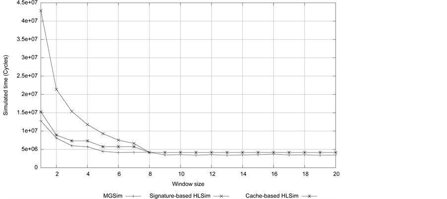
The simulated time of the Livermore kernel 7 (LMK7) of size 99,000 on different simulators on different number of cores is shown in Figure 9. LMK7 is a memory intensive application. We can see that, on cores 20 to cores 23, Cache-based HLSim is more accurate than Signature-based HLSim. This accuracy is not clear when we use larger window size (as shown in the above experiments), but we clearly see the difference in accuracy with small number of active threads. With cores 24, and cores 25, simulated time is not reduced in MGSim. It is assumed to be the pressure on the memory channels. It can be seen that both HLSim models predict the same maximum window size for this application as MGSim, i.e. 8 for up to 8 cores. However for larger number of cores, although the two models are consistent, they over-estimate the window size compared to MGSim.
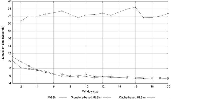
The simulation time of LMK7 on different simulators on different number of cores is shown in Figure 10. We clearly see that Signature-based HLSim and Cache-based HLSim are few orders of magnitude faster than MGSim. The important conclusion from this experiment is that, despite increasing the accuracy in Cache-based HLSim, the simulation time remains close to Signature-base HLSim. This indicates, that our improved simulation technique does not affect the simulation time (if we ignore the setup of the database).
In order to demonstrate further that we have a clear difference in the accuracy of different levels of HLSim when small number of threads are active in the pipeline, we execute FFT of size 28 on cores 23 by choosing different window sizes in the range of 1 to 16 in MGSim and different levels of HLSim and this is shown in Figure 11. It should also be noted that window size only restricts the number of threads created per family and is not necessarily a representation of the number of active threads in the pipeline. In the figure, the X-axis shows window size and Y-axis shows simulated time. One-IPC HLSim shows a straight line as expected, because the throughput is never adapted by the number of threads and it is assumed that all instructions execute in a single cycle. Signature-based HLSim adapts the throughput based on the latency factor model, but the accuracy is not as close to MGSim as Cache-based HLSim, because the access to different levels of cache is not considered. Cache-based HLSim gives the best fidelity, especially when there are small number of active threads. With the increased number of active threads (after 8 window size in this experiment) Signature-based HLSim and Cache- based HLSim converge. Analytical-based HLSim achieves the maximum possible accuracy, because the throughput is taken from the look up table which is filled with empirical data derived from MGSim. It should be noted that window size does not show the exact number of active threads in pipeline.
In this experiment the optimal window size for FFT, given by MGSim is 4, whereas both Signature and Cache-based HLSim predict a slight improvement at 8 threads. Again both models predict the same optimal window size although again this is overestimated by a factor of 2. The gradual increase in execution time in MGSim after 4 threads is probably because of waiting for synchronisation on writes, which is not taken account of in both HLSim models.
7.6. IPC-Simulation Accuracy
Simulated instructions Per Cycle (IPC) is an indirect measure of efficiency in the Microgrid with its data flow scheduling as there is no busy waiting on synchronisation. For each core the IPC should be as close to the number of instructions the architecture is capable of issuing in each cycle. In the case of the Microgrid, with single issue, the IPC of each core should be as close to 1 as possible. However, for c cores, the overall IPC may be up to c, i.e. each core may issue 1 instruction per cycle. We can also measure the average IPC, i.e. sum the IPC of c cores and divide by c.
 (a)
(a) (b)
(b) (c)
(c) (d)
(d) (e)
(e)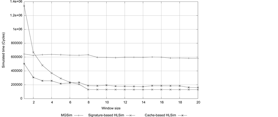 (f)
(f)
Figure 9. Simulated time of LMK7 of size 99,000 using different window sizes in MGSim, Signature-based HLSim and Cache-based HLSim. (a) Simulated time on 20 core; (b) Simulated time on 21 cores; (c) Simulated time on 22 cores; (d) Simulated time on 23 cores; (e) Simulated time on 24 cores; (f) Simulated time on 25 cores.
 (a)
(a) (b)
(b) (c)
(c) (d)
(d) (e)
(e)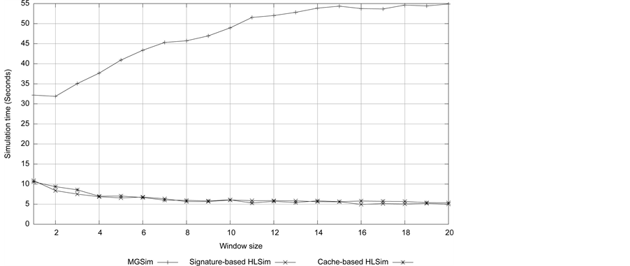 (f)
(f)
Figure 10. Simulation time of LMK7 using different window sizes in MGSim, Signature-based HLSim and Cache-based HLSim. (a) Simulation time on 20 core; (b) Simulation time on 21 core; (c) Simulation time on 22 core; (d) Simulation time on 23 core; (e) Simulation time on 24 core; (f) Simulation time on 25 core.

Figure 11. The effect of changing the window size on the execution of FFT of size 28 and cores 23 using MGSim and different levels of HLSim.

Figure 12. IPC across different number of simulated cores in selected applications using MGSim and different levels of HLSim. (a) IPC in MGSim; (b) IPC in One-IPC HLSim; (c) IPC in Signature-based HLSim; (d) IPC in Cache-based HLSim.
The IPC using different number of cores for MGSim and different levels of HLSim is shown in Figure 12 for a range of applications. These graphs show the IPC of different simulators individually for different number of cores. In MGSim instructions take longer time to complete e.g. floating point operations or memory operations take more than one cycles when there is no latency tolerance. There are other issues such as load balancing that reduce the IPC on more than one core. Therefore total instructions executed per cycle on average is lower than one. One-IPC HLSim executes all instructions as one instruction per cycle, therefore the IPC is one on different number of cores. In Signature-based HLSim and Cache-based HLSim, instructions are classified by latency and execution rate is adapted based on the number of active threads, therefore the IPC is lower than one.
We show the average IPC (averaged across different simulated cores) in MGSim and different levels of HLSim in Figure 13. One-IPC HLSim has 1 IPC all the time, as expected. In Gol (Grids), FFT, LMK7 and Mandelbrot, the IPC of Cache-based HLSim is closer to MGSim. This shows the relative accuracy of Cache- based HLSim compared to Signature-based HLSim.
In some applications MGSim is efficient in others not, because of the pressure on memory and load balancing. The IPC in HLSim depends on the abstraction over the detailed instruction execution in MGSim. We see that the IPC of different levels of HLSim is not uniform across all the applications, when compared to the IPC achieved in MGSim. We can rely on instruction counting in HLSim, but their abstraction and the dynamic adaptation depends on the distribution of instructions and the state of the system. Therefore the IPC will not be fixed in comparison to MGSim. We can see this direct comparison in computing the percentage error of different levels of HLSim to MGSim and this is shown in Table 1. In GOL (Torus) and Mandelbrot, One-IPC HLSim has less percent error in comparison to Signature-based HLSim and Cache-based HLSim. Signature-based HLSim is more accurate compared to Cache-based HLSim in Gol(Torus), MatrixMultiply and Smooth. In the other applications Cache-based HLSim has less percentage error than any other level of the HLSim.
7.7. IPS-Simulation Speed
Instructions per second (IPS) is used to measure the basic performance of an architecture. It is an interesting measure in simulation as we can use it to measure the simulated instructions per second using a known contem-

Figure 13. Average IPC of different cores in MGSim and different levels of HLSim.

Table 1. Percent error in the average IPC of different cores in MGSim and different levels of HLSim.
porary processor and determine the overall simulation speed of the architecture.
In this experiment we want to calculate the IPS of different levels of HLSim and MGSim. Although we know that the IPS of MGSim is 100KIPS (Kilo Instructions Per Second), we would like to recompute the IPS for MGSim in selected applications and compare with the IPS of HLSim. In our experiments, IPS is computed as the number of simulated instructions divided by the simulation time over the program execution. The IPS of a simulator depends on the configuration of the host machine and the simulator, which we have given in Section 7.1. We show the IPS in selected applications per different simulated cores for MGSim, One-IPC HLSim, Signature-based HLSim and Cache-based HLSim in Figures 14(a)-(d) respectively. These graphs show the IPS of different simulators individually. We have explained that Signature-based HLSim and Cache-based HLSim has high accuracy compared to One-IPC HLSim, but all of these levels show the same simulation speed.
In order to compare the IPS across different simulators, we take the average of IPS across different number of simulated cores in all selected applications. The average IPS for each application is shown in Figure 15. The average IPS of different levels of HLSim remains the same, but higher than the IPS in MGSim.
To show the combined IPS of different simulators based on the selected applications, we can take another average across all applications. The average IPS for HLSim is 925KIPS and the average IPS for MGSim is 170KIPS. The 170KIPS of MGSim is close to 100KIPS as advertised. Based on the given experiments we can present that HLSim is a 1MIPS (Mega Instructions Per Second) simulator.
 (a)
(a)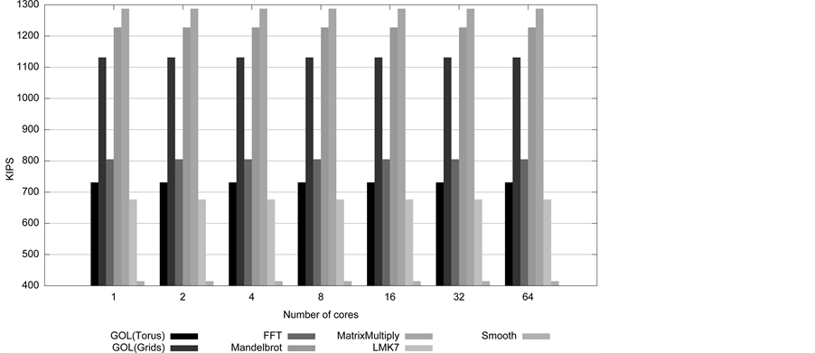 (b)
(b) (c)
(c) (d)
(d)
Figure 14. IPS across different number of simulated cores in selected applications using MGSim and different levels of HLSim. (a) IPS in MGSim; (b) IPS in One-IPC HLSim; (c) IPS in Signature-based HLSim; (d) IPS in Cache-based HLSim.

Figure 15. The average IPS of different simulated cores across a range of applications in MGSim and different levels of HLSim.
Different simulators used in industry and academia with their simulation speed in terms of IPS are; COTSon [21] executes at 750KIPS, SimpleScalar [20] executes at 150KIPS and Interval simulator [2] executes at 350KIPS. MGSim [7] executes at 100KIPS. Compared to the IPS of these simulators the IPS of HLSim is very promising. It should be noted that the IPS of simulation frameworks given above are simulating only few number of cores on the chip. In MGSim and HLSim we have simulated 128 cores on a single chip. Given this large number of simulated cores on a chip, 1MIPS indicates a high simulation speed.
IPS in Analytical-based HLSim: The IPS of Front-end HLSim and Analytical-based HLSim are not presented previously. In Front-end HLSim we do not simulate instructions at all. In Analytical-based HLSim, we map the throughput of the program from the database to the signature in HLSim. These signatures are counted as simulated instructions, and then we map this throughput to the architecture model to advance the simulated time. This does not give us an exact IPS for analytical-based HLSim, but we can compute an equivalent IPS shown in Figure 16. The X-axis shows the number of simulated cores, and the Y-axis shows the GIPS (Giga Instructions per Second). Based on this experiment we can claim that the IPS of Analytical-based HLSim is 100 GIPS (Giga Instructions Per Second). It should be noted that Analytical-based HLSim may not be used stand alone, but as part of a large simulation when doing design space exploration. Therefore the cost of obtaining the analytical results using MGSim are amortised across many runs of a component, e.g. FFT may be executed many times in a large complex simulation and indeed used in many applications.
8. Related Work
High-level simulators have been used for DSE in the embedded systems domain for more than a decade, and are used in the research in both academia and industry. Some of the research groups using high-level simulation for DSE in embedded systems are; (Metro) Polis [31] , Mescal [32] , Milan [33] , The octopus toolset [34] and SystemC-based environment developed at STMicroelectronics [35] . However, the use of high-level simulators for DSE in general-purpose, multi- and many-core systems is a relatively new research domain. In this section we give high-level simulation techniques for the general-purpose computers.
Interval simulation [2] [36] is a high-level simulation technique for the DSE of super-scalar single- and multi- core processors. It raises the level of abstraction from detailed simulation by using analytical models to derive the timing simulation of individual cores without the detailed execution of instructions in all the stages of the pipeline. The model is based on deriving the execution of an instruction stream in intervals. An interval is decided based on a miss event, e.g. branch misprediction, cache misses, TLB misses etc. With interval analysis, execution time is partitioned into discrete intervals using these miss events. The analytical models of every core

Figure 16. IPS across different number of simulated cores in selected applications using analytical-based HLSim.
cooperate with miss events in the system and can be extended to model the tight interleaving of threads in multi-core processors.
Nussbaum and Smith [37] and Hughes and Li [38] use statistical simulation paradigm to multi-threaded programs running on shared-memory multiprocessor (SMP) systems. They have extended the statistical simulation to model synchronization and accesses to shared memory. Genbrugge and Eeckhout [39] [40] use statistical simulation to measure some execution characteristics in the statistical profile to be able to accurately simulate shared resources in multi-core processors.
Different research in multi-threaded and multi-core processors simulation is using sampled simulation. Van Biesbrouck et al. [41] propose the co-phase matrix for speeding up sampled simultaneous multithreading (SMT) processor simulation running multi-program workloads. Stenstrom et al. [42] researching that fewer sampling units are enough to estimate overall performance for larger multi-processor systems than for smaller multi-processor system in case one is interested in aggregate performance only. Wenisch et al. [43] have obtained similar conclusions of throughput in server workloads. Barr et al. [44] proposes the Memory Time-stamp Re- cord (MTR) to store micro-architecture state (cache and directory state) at the beginning of the sampling unit as a checkpoint.
9. Discussion
In this section we give an overview of the lessons learned from the research presented in this paper.
9.1. Microgrid vs. Many-Cores
We have presented different levels of HLSim in the context of the Microgrid. However, these simulation techniques are more general and can be used for developing high-level simulators for other many-core systems. Such systems are likely to use large number of cores on a single chip. Some cores have hardware threads for fine-grained latency tolerance others not. Intel SCC, does not have hardware threads and therefore the throughput of the program is not required to be adapted based on the number of threads in the pipeline, we can use the architecture modelling technique in One-IPC HLSim.
The UltraSPARC series of processors have hardware threads to achieve latency tolerance in long latency operations. Similarly TILE64 provides fine-grained latency tolerance. These architectures require dynamic adaptation based on the type of instruction, number of instructions and active threads. Therefore the simulation techniques presented in Signature-based HLSim can be used. In case more accuracy is desired, then Cache-based HLSim simulation techniques can also be used.
The performance estimation technique presented in Signature-based HLSim is an efficient source-based technique and can be used in embedded systems or general purpose systems for performance estimation. Similarly the high-level cache modelling is a novel simulation technique, and can be used in many-core systems for the distributed memory architectures with cache coherency protocols.
In the Microgrid, cores are single issue, and based on RISC, which are abstracted in HLSim. However, even if the underlying core is different i.e. based on CISC or has multiple issues in the pipeline etc. the high-level simulation techniques presented in this paper can still be applicable. Because, in the high-level simulation, we show how we abstracted the simulated time from the execution of instructions in detailed in the pipeline of the core. Similarly, we can abstract the details in more complicated cores, and once we have the abstracted simulated time, we can use the high-level simulation techniques presented in this paper.
9.2. Simulation Speed
High simulation speed is desired in high-level simulation in order to perform design space exploration. But HLSim is based on pthreads, where the host machine is involved in creation, termination and synchronization of the threads which are limited by the host machine and address space available in the system. We are also using mutexes in the high-level simulator, which reduces the performance of the application on multi-core and many-core machines. This means that in the current implementation we have achieved only 10 times improvement in Front-end HLSim compared to MGSim. One-IPC HLSim has added overhead, because threads in the application models are blocked until their events are serviced by a single thread representing the architecture model. However, it is important to note that the other levels of HLSim i.e. Signature-based HLSim and Cache- based HLSim do not affect the simulation speed significantly, while improving the accuracy compared to One-IPC HLSim. Analytical-based HLSim shows the highest possible simulation speed, when the blocking, synchronization, creation and termination operations of POSIX threads are removed. Therefore we can claim that the high-level simulation techniques presented in the research of this paper can exhibit the highest simulation speed given that the underlaying framework has a high simulation speed.
HLSim was initially based on pthreads because pthreads provide constructs that were used as straight forward transformation of the microthreading model. At the time we started to work on HLSim, we wanted to produce results to evaluate the design of the Microgrid and to be able to evaluate microthreaded programs in a high-level language, and pthreads was the straight forward option with the least development effort. The implementation of the microthreaded model in pthreads and later the different levels in the high-level simulation has saved us development time from investigating other more complex approaches. The high-level simulator is less complex, reasonably accurate but its simulation speed depends on the efficient execution of pthreads on the host machine.
Bluespec [45] is a simulation technology that has evolved over the years. It has dramatically lowered the cost of low-level simulation, by enabling the designer to use a specification language that is very high-level. In addition, Bluespec provides the easy transformation from system-level specification to VHDL simulation. This way a huge amount of effort can be saved in transition from one level to another level. Moreover, Bluespec provides reduced complexity in simulation. At the time the research on HLSim was started, Bluespec was not a mature technology, and therefore was never used in our research. But with the advancement of this technology, we believe that we can achieve higher simulation speeds if we re-write our simulation framework in Bluespec. However, until Bluespec is proven to make a decisive difference in cost, we also probably want to use high-level simulation techniques.
In summary, there are qthreads [46] , which can create ten of thousands of threads without too much cost of creation and synchronization. There are also other frameworks that provide “lightweight” threads. We are using pthreads, because the application model of HLSim was already tested to be executed on multiple platforms using this technology. We, did not want to spend time on the application model, but rather investigate the architecture model and hence the Microgrid platforms. The good news is that, we have presented multiple levels of abstractions in the simulation, which can be used irrespective of the changes in the underlying threading environment and without significant overhead on top of the application model’s execution.
9.3. Simulation Accuracy
In Section 7.4, we observed that we have an inaccuracy in HLSim for large window sizes. But, we see that when we have a smaller number of active threads, then we show that accuracy across different levels of HLSim changes. We have three different hypothesis for the inaccuracy:
1) The first was register-file constraints. However, we have adapted the window size in HLSim to restrict the number of threads in HLSim to match the constraints in MGSim (Section 7.4). Even then we have observed that we do not see any improvement in the accuracy of HLSim when the window size is larger than the length of the pipeline. Because, in HLSim, once the number of active threads increases then the length of the pipeline, the latency factors reduce to 1 or 2 and hence we do not see any further improvement in accuracy. It should also be noted that window size does not represent the total number of simultaneous active threads during the execution of the program.
2) We know that stores impact the cost of synchronisation in MGSim hence degrading performance [47] . However, we do not know how much impact it can have on the inaccuracy of HLSim.
3) We have taken an average of the cache statistics in Cache-based HLSim. However, some applications like FFT have very different characteristics in different stages of the application. For example in the early stages, FFT has good cache locality and in the latter stages it has very poor cache locality. This may also have an impact on HLSim accuracy.
10. Conclusion
Simulations are commonly used during the design of computer architectures. Different simulators are developed, with different complexity, simulation speed, accuracy and development time. Computer architects are always looking for simulation techniques that are useful for design space exploration. These simulators are required to have reduced complexity, short development time and high simulation speed, with the only compromise being a loss of accuracy in the simulation. These simulators are known as high-level simulation and are useful tools in the designer’s toolbox for design space exploration. In this paper, we presented multiple levels of the high-level simulator for a particular implementation of a many-core system i.e. Microgrid. We demonstrated that based on the requirement of accuracy and the detail of the exploration of the architecture a level of HLSim can be used. It is also important to note that, despite increasing the accuracy, the simulation speed is not affected. We have demonstrated that the high-level simulation technique presented in this paper can achieve the highest possible simulation speed, given that the underlying framework can support faster execution of threads.
Acknowledgements
This research work was carried out at University of Amsterdam, the Netherlands.
Cite this paper
IrfanUddin, (2015) Multiple Levels of Abstraction in the Simulation of Microthreaded Many-Core Architectures. Open Journal of Modelling and Simulation,03,159-190. doi: 10.4236/ojmsi.2015.34017
References
- 1. Uddin, I. (2013) Design Space Exploration in the Microthreaded Many-Core Architecture. University of Amsterdam, arXiv Technical Report.
http://arxiv.org/abs/1309.5551 - 2. Carlson, T.E., Heirman, W. and Eeckhout, L. (2011) Sniper: Exploring the Level of Abstraction for Scalable and Accurate Parallel Multi-Core Simulation. Proceedings of 2011 International Conference for High Performance Computing, Networking, Storage and Analysis, ACM, New York, 1-12.
http://dx.doi.org/10.1145/2063384.2063454 - 3. Jesshope, C.R. (2006) Microthreading a Model for Distributed Instruction-Level Concurrency. Parallel Processing Letters, 16, 209-228.
http://dx.doi.org/10.1142/S0129626406002587 - 4. Uddin, I. (2013) Microgrid—The Microthreaded Many-Core Architecture. University of Amsterdam, arXiv Technical Report.
http://arxiv.org/abs/1309.5507 - 5. Bernard, T.A.M., Grelck, C., Hicks, M.A., Jesshope, C.R. and Poss, R. (2011) Resource-Agnostic Programming for Many-Core Microgrids. Proceedings of the 2010 Conference on Parallel Processing, Springer-Verlag, Berlin, Heidelberg, 109-116.
http://dl.acm.org/citation.cfm?id=2031978.2031994 - 6. van Tol, M., Jesshope, C., Lankamp, M. and Polstra, S. (2009) An Implementation of the Sane Virtual Processor Using Posix Threads. Journal of Systems Architecture, 55, 162-169.
http://www.sciencedirect.com/science/article/B6V1F-4TS6STP-1/2/82465c0360291ccf954008ae85c7331b - 7. Bousias, K., Guang, L., Jesshope, C.R. and Lankamp, M. (2009) Implementation and Evaluation of a Microthread Architecture. Journal of Systems Architecture, 55, 149-161.
http://dl.acm.org/citation.cfm?id=1517865.1518255 - 8. Kena Poss, R. (2012) SL—A “Quick and Dirty” but Working Intermediate Language for SVP Systems. University of Amsterdam, Technical Report.
http://arxiv.org/abs/1208.4572 - 9. Poss, R., Lankamp, M., Yang, Q., Fu, J., Uddin, I. and Jesshope, C. (2013) MGSim—A Simulation Environment for Multi-Core Research Education. SAMOS.
http://dx.doi.org/10.1109/samos.2013.6621109 - 10. Kena Poss, R., Lankamp, M., Yang, Q., Fu, J., van Tol, M.W., Uddin, I. and Jesshope, C.R. (2013) Apple-CORE: Harnessing General-Purpose Many-Cores with Hardware Concurrency Management. Microprocessors and Microsystems.
http://www.sciencedirect.com/science/article/pii/S0141933113000835 - 11. Poss, R., Lankamp, M., Uddin, I., Sykora, J. and Kafka, L. (2012) Heterogeneous Integration to Simplify Manycore Architecture Simulations. Proceedings of the 2012 Workshop on Rapid Simulation and Performance Evaluation: Methods and Tools, Ser. RAPIDO ’12, ACM, New York, 17-24.
- 12. Uddin, I. (2009) High-Level Simulation of the Microgrid. Master’s Thesis, University of Amsterdam, Amsterdam.
http://www.scriptiesonline.uba.uva.nl/313593 - 13. Uddin, I., van Tol, M.W. and Jesshope, C.R. (2011) High-Level Simulation of SVP Many-Core Systems. Parallel Processing Letters, 21, 413-438.
http://www.worldscinet.com/ppl/21/2104/S0129626411000308.html - 14. Lankamp, M., Poss, R., Yang, Q., Fu, J., Uddin, I. and Jesshope, C.R. (2013) MGSim—Simulation Tools for Multicore Processor Architectures. University of Amsterdam, Technical Report.
http://arxiv.org/abs/1302.1390 - 15. Kienhuis, B., Deprettere, E.F., Wolf, P.V.D. and Vissers, K.A. (2002) A Methodology to Design Programmable Embedded Systems—The y-Chart Approach. Embedded Processor Design Challenges: Systems, Architectures, Modeling, and Simulation—AMOS, Springer-Verlag, London, 18-37.
http://dl.acm.org/citation.cfm?id=646466.691571 - 16. Bolychevsky, A., Jesshope, C.R. and Muchnick, V.B. (1996) Dynamic Scheduling in Risc Architectures. IEEE Proceedings Computers and Digital Techniques, 143, 309-317.
http://dx.doi.org/10.1049/ip-cdt:19960788 - 17. Uddin, I., Poss, R. and Jesshope, C. (2014) Analytical-Based High-Level Simulation of Microthreaded Many-Core Architectures. PDP.
- 18. Thompson, M. (2012) Tools and Techniques for Efficient System-Level Design Space Exploration. Ph.D. Dissertation, University of Amsterdam.
- 19. Bernard, T.A.M., Bousias, K., Guang, L., Jesshope, C.R., Lankamp, M., van Tol, M.W. and Zhang, L. (2008) A General Model of Concurrency and Its Implementation as Manycore Dynamic Risc Processors. ICSAMOS’08, 1-9.
- 20. Austin, T., Larson, E. and Ernst, D. (2002) SimpleScalar: An Infrastructure for Computer System Modeling. Computer, 35, 59-67.
http://dx.doi.org/10.1109/2.982917 - 21. Argollo, E., Falcon, A., Faraboschi, P, Monchiero, M. and Ortega, D. (2009) Cotson: Infrastructure for Full System Simulation. ACM SIGOPS Operating Systems Review, 43, 52-61.
http://dx.doi.org/10.1145/1496909.1496921 - 22. Rosenblum, M., Bugnion, E., Devine, S. and Herrod, S.A. (1997) Using the SimOS Machine Simulator to Study Complex Computer Systems. ACM Transactions on Modeling and Computer Simulation, 7, 78-103.
http://dx.doi.org/10.1145/244804.244807 - 23. Magnusson, P.S., Christensson, M., Eskilson, J., Forsgren, D., Hallberg, G., Hogberg, J., Larsson, F., Moestedt, A. and Werner, B. (2002) Simics: A Full System Simulation Platform. Computer, 35, 50-58.
http://dx.doi.org/10.1109/2.982916 - 24. Daněk, M., Kafka, L., Kohout, L., Sykora, J. and Bartosinski, R. (2012) UTLEON3: Exploring Fine-Grain Multi-Threading in FPGAs, Ser. Circuits and Systems. Springer.
- 25. Uddin, I. (2015) One-Ipc High-Level Simulation of Microthreaded Many-Core Architectures. International Journal of High Performance Computing Applications.
http://dx.doi.org/10.1177/1094342015584495 - 26. Uddin, I., Poss, R. and Jesshope, C. (2014) Signature-Based High-Level Simulation of Microthreaded Many-Core Architectures. SIMULECH.
http://dx.doi.org/10.5220/0004982405090516 - 27. Uddin, I., Jesshope, C.R., van Tol, M.W. and Poss, R. (2012) Collecting Signatures to Model Latency Tolerance in High-Level Simulations of Microthreaded Cores. Proceedings of the 2012 Workshop on Rapid Simulation and Performance Evaluation: Methods and Tools, Ser. RAPIDO ’12, ACM, New York, 1-8.
http://dx.doi.org/10.1145/2162131.2162132 - 28. Uddin, I., Poss, R. and Jesshope, C. (2014) Cache-Based High-Level Simulation of Microthreaded Many-Core Architectures. Journal of Systems Architecture, 60, 529-552.
http://www.sciencedirect.com/science/article/pii/S1383762114000812 - 29. Keutzer, K., Malik, S., Member, S., Newton, A.R., Rabaey, J.M. and Sangiovanni-Vincentelli, A. (2000) System-Level Design: Orthogonalization of Concerns and Platformbased Design. IEEE Transactions on Computer-Aided Design of Integrated Circuits and Systems, 19, 1523-1543.
http://dx.doi.org/10.1109/43.898830 - 30. Misra, J. (1986) Distributed Discrete-Event Simulation. ACM Computing Surveys, 18, 39-65.
http://dx.doi.org/10.1145/6462.6485 - 31. Yang, G. Parallel Simulation in Metropolis.
- 32. Denneulin, Y. Mescal. http://mescal.imag.fr/collab-acad-nat.php
- 33. Bakshi, A. and Ledeczi, A. (2001) Milan: A Model Based Integrated Simulation Framework for Design of Embedded Systems. ACM SIGPLAN Notices, 82-93.
http://dx.doi.org/10.1145/384196.384210 - 34. Basten, T., Van Benthum, E., Geilen, M., Hendriks, M., Houben, F., Igna, G., Reckers, F., De Smet, S., Somers, L., Teeselink, E., Trcka, N., Vaandrager, F., Verriet, J., Voorhoeve, M. and Yang, Y. (2010) Model Driven Design-Space Exploration for Embedded Systems: The Octopus Toolset. Proceedings of the 4th International Conference on Leveraging Applications of Formal Methods, Verification, and Validation, Ser. ISoLA’10, Springer-Verlag, Berlin, Heidelberg, 90-105.
http://dl.acm.org/citation.cfm?id=1939281.1939293 - 35. Wellig, A. and Zory, J. (2003) Framed Complexity Analysis in Systemc for Multi-Level Design Space Exploration. Proceedings of the Euromicro Symposium on Digital System Design, 416-423.
http://dx.doi.org/10.1109/dsd.2003.1231975 - 36. Genbrugge, D., Eyerman, S. and Eeckhout, L. (2010) Interval Simulation: Raising the Level of Abstraction in Architectural Simulation. HPCA, 1-12.
- 37. Nussbaum, S. and Smith, J.E. (2002) Statistical Simulation of Symmetric Multiprocessor Systems. SS’02: Proceedings of the 35th Annual Simulation Symposium, IEEE Computer Society, Washington DC, 89.
http://dx.doi.org/10.1109/simsym.2002.1000093 - 38. Hughes, C. and Li, T. (2008) Accelerating Multi-Core Processor Design Space Evaluation Using Automatic Multi-Threaded Workload Synthesis. 2008 IEEE International Symposium on Workload Characterization, 163-172.
http://dx.doi.org/10.1109/IISWC.2008.4636101 - 39. Eeckhout, L., Nussbaum, S., Smith, J.E. and Bosschere, K.D. (2003) Statistical Simulation: Adding Efficiency to the Computer Designer’S Toolbox. IEEE Micro, 23, 26-38.
http://dl.acm.org/citation.cfm?id=1435585.1435761 - 40. Genbrugge, D. and Eeckhout, L. (2009) Chip Multiprocessor Design Space Exploration through Statistical Simulation. IEEE Transactions on Computers, 58, 1668-1681.
http://dx.doi.org/10.1109/TC.2009.77 - 41. Van Biesbrouck, M., Sherwood, T. and Calder, B. (2004) A Cophase Matrix to Guide Simultaneous Multithreading Simulation. Proceedings of the 2004 IEEE International Symposium on Performance Analysis of Systems and Software, Ser. ISPASS ’04, IEEE Computer Society, Washington DC, 45-56.
http://dl.acm.org/citation.cfm?id=1153925.1154587 - 42. Ekman, M. and Stenstrom, P. (2005) Enhancing Multiprocessor Architecture Simulation Speed Using Matchedpair Comparison. Proceedings of the IEEE International Symposium on Performance Analysis of Systems and Software, Ser. ISPASS’05, IEEE Computer Society, Washington DC, 89-99.
- 43. Wenisch, T.F., Wunderlich, R.E., Ferdman, M., Ailamaki, A., Falsafi, B. and Hoe, J.C. (2006) Simflex: Statistical Sampling of Computer System Simulation. IEEE Micro, 26, 18-31.
http://dx.doi.org/10.1109/MM.2006.79 - 44. Barr, K.C., Pan, H., Zhang, M. and Asanovic, K. (2005) Accelerating Multiprocessor Simulation with a Memory Timestamp Record. Proceedings of the IEEE International Symposium on Performance Analysis of Systems and Software, Ser. ISPASS’05, IEEE Computer Society, Washington DC, 66-77.
http://dx.doi.org/10.1109/ispass.2005.1430560 - 45. Bluespec. The Synthesizable Modeling Company. Fast, Early and Accurate. http://www.bluespec.com
- 46. Qthreads—Lightweight Locality-Aware User-Level Threading Runtime. http://code.google.com/p/qthreads/
- 47. Yang, Q. and Jesshope, C.R. (2013) On-Chip Memory Traffic Regulation for the Microgrid. ACM Transactions on Embedded Computing Systems (TECS).