Open Journal of Modelling and Simulation
Vol.1 No.3(2013), Article ID:34306,6 pages DOI:10.4236/ojmsi.2013.13006
A Boundary Element Formulation for the Pricing of Barrier Options
1Institute of Applied Mathematics, National Cheng-Kung University, Taiwan
2Department of Finance, National Dong Hwa University, Taiwan.
Email: shen@mail.ncku.edu.tw, hsiao@mail.ndhu.edu.tw
Copyright © 2013 Shih-Yu Shen, Yi-Long Hsiaoy. This is an open access article distributed under the Creative Commons Attribution License, which permits unrestricted use, distribution, and reproduction in any medium, provided the original work is properly cited.
Received March 13, 2013; revised April 25, 2013; accepted May 1, 2013
Keywords: Boundary Element Method; Black-Scholes Equation; Moving Boundary; Option Pricing; Barrier Option
ABSTRACT
In this article, we derive a boundary element formulation for the pricing of barrier option. The price of a barrier option is modeled as the solution of Black-Scholes’ equation. Then the problem is transformed to a boundary value problem of heat equation with a moving boundary. The boundary integral representation and integral equation are derived. A boundary element method is designed to solve the integral equation. Special quadrature rules for the singular integral are used. A numerical example is also demonstrated. This boundary element formulation is correct.
1. Introduction
Boundary element methods are efficient for solving linear partial differential equation. In this paper we discuss a boundary element formulation for the pricing of barrier options. An option which is activated or deactivated once the price of the underlying asset reaches a set level is called a barrier option. The predetermined level is called the barrier. There are two types of barrier options, “in” and “out” options. A barrier option is said to be of knock-out type, if the option is de-activated when the stock price hit the barrier.A payment (the rebate) may be made when a knock-out barrier option is de-activated. The rebate amount may depend on the time of hitting. A barrier option is said to be of knock-in type if the option is activated upon hitting. Barrier options are path-dependent exotics. Although our method can be applied on both types, we formulate the method for knock-out call. A knock-out call with constant barrier and zero rebate is easy to price. In this study, we deal with options with time-varied barrier and non-zero rebate.
Since the publication of Black and Scholes’ [1], and Merton’s [2] papers in 1973, the Black-Scholes model has become the preferred framework for option pricing. In the Black-Scholes model, the option price is considered as a function of stock price and time. The option price  can be obtained by solving the BlackScholes equation. In 1979, Cox, Ross and Rubinstein [3]
published a paper detailing how the option price can be obtained by evaluating the expected value. Since then, most researchers use probability methods to price options. Some researchers report pricing barrier options by using probability methods as outlined in the literature. For example, Kunitomo and Ikeda [4] used a serial solution for the probability of the asset price reaching in an interval at the maturity without hitting curved boundaries. As a result, the expected value of the option could be obtained. Geman and Yor [5] followed Kunitomo and Ikeda’s method but used Laplace transform to simplify the formulation, while Plesser [6] also followed the same arguments but used contour integral to calculate the inverse Laplace transform. In this study, we solve the BlackScholes equation to obtain the barrier option price.
The Black-Scholes equation is a non-homogeneous linear partial differential equation (PDE). Pricing plain options only needs to solve the initial value problem. However, pricing barrier options and some other exotic options necessitate solving initial-boundary value problems. Domain type numerical methods, such as finite difference method and finite element method, are used to solve these kinds of problems, as in [7-9]. Using a set of variable transformations, the Black-Scholes equation can be converted into a homogeneous linear PDE, i.e., a heat equation. Arguably, the boundary element method (BEM) may be the best numerical method for pricing double barrier options. BEMs are rarely applied to financial problems, although Shen and Wang used a BEM to evaluate the expected value of stock price [10].
A stock option represents a contract where the holder is endowed with the right, but not the obligation, to buy or sell a fixed number of shares of a specified common stock at a specific price on or before a certain date. A call option endows the holder with the right to buy the shares, and a put option endows the holder with the right to sell the shears. The stock, the specific price and the certain date are called the underlying asset, the exercise price and the maturity date respectively. In this paper, the price of a barrier option is modeled as a solution of the boundary value problem, and a boundary element method is designed to solve the problem. The outline of the paper is arranged as follows. In Section 2, we introduce the mathematical model of the knock-out call option. The resulting problem is a boundary value problem of a heat equation. In Section 3, the integral representations of the solution of the boundary value problem are derived. An effective boundary element method is designed to solve the boundary value problem in the following section. In Section 5, we show the results of a simple example. The results show the formulation is correct. The last section is a short conclusions.
2. The PDE and the Boundary Conditions
A knock-out call has a barrier. When the stock price touches the barrier, the option becomes null and the option writer may pay the immediate rebate to the option holder. Hence, the value of the option is determined when the stock price touches the barrier. If the stock price does not touch the barrier before maturity, the holder may exercise his/her options with the exercise price at maturity.
We follow the arguments of Black and Scholes [1]. The call option price  satisfies the Black-Scholes equation,
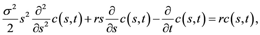 (1.1)
(1.1)
where ![]() is the underlying asset price,
is the underlying asset price,  is the time to maturity,
  is the risk-free interest rate, and
 ![]() is the volatility of the underlying asset price.
is the volatility of the underlying asset price.
At maturity, the payoff of the option has to be the maximum of  and 0, where
  is the exercise price. Therefore, the initial condition is
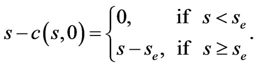 (1.2)
(1.2)
When the underlying asset price touches the predetermined barrier  at the time to maturity
 , the option holder will receive the immediate rebates
 . Hence, the boundary conditions are
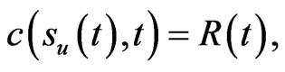 (1.3)
(1.3)
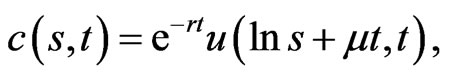
A set of variable transformations is used to simplify the mathematical problem. Let
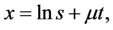 (1.4)
(1.4)
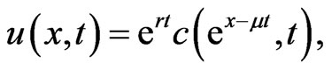 (1.5)
(1.5)
where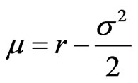 . The Black-Scholes equation will be transformed to a heat equation,
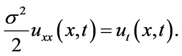 (1.6)
(1.6)
The initial condition becomes
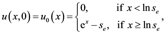 (1.7)
(1.7)
and the new boundary conditions are
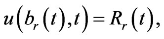 (1.8)
(1.8)
where the transformations of the barrier and rebate are
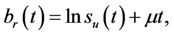 (1.9)
(1.9)
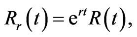 (1.10)
The PDE (1.6), the initial condition (1.7) and the boundary conditions (1.8) compose a well-posed boundary value problem. In the following sections, we derive the boundary integral equation and solve the equation numerically.
3. The Integral Representation
The solution of the boundary value problem can be formulated by an integral representation. We describe the integral representation briefly and then perform a limiting process to obtain the boundary integral equations in this section. Let  be a fundamental solution of the dual equation of Equation (1.6), that is
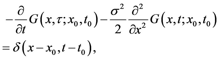 (1.11)
where  is the 2-D Dirac delta function. There is a fundamental solution
 ,
,
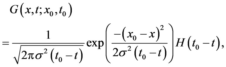 (1.12)
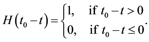
where  is the Heviside step function,
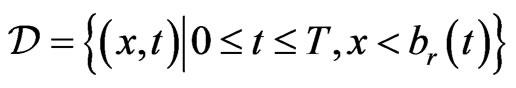
Since  fulfills Equation (1.6) in domain
 we have
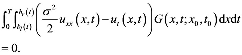 (1.13)
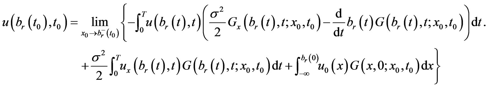
Applying the integration by parts on Equation (1.13), we obtain the integral representation for the point 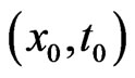 in domain
 . The integral representation is
 (1.14)
Because the solution  is continuous on the set
 ,
, 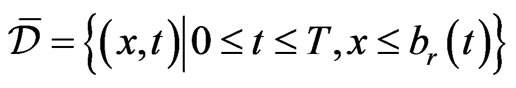 , the limit has to be the boundary value when the point
  approaches the boundary point
 , that is
 (1.15)
Be noted that
 (1.16)
where the principal value integral is defined as
 (1.17)
Therefore, Equation (1.15) becomes
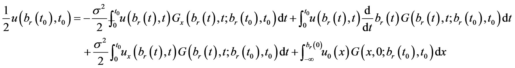 (1.18)
In Equations (1.18),  is unknown function. For convenience, let
 (1.19)
Substituting the boundary conditions (1.8) into Equation (1.18), we obtain Equation (1.20).
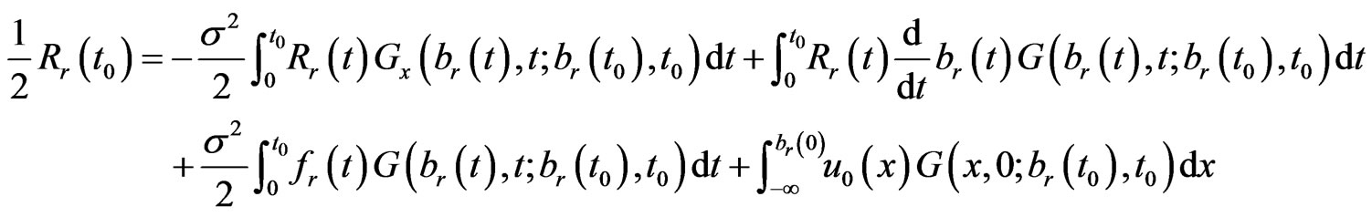 (1.20)
Equation (1.20) is the boundary integral equation for the unknown function .
.
4. Boundary Element Formulation
In this section, a boundary element method is designed to solve the moving boundary value problem. In order to evaluate , the function
  of Equation (1.20) have to be solved first.
We consider that the problem has to be solved on the time interval . To start the discretization, the time interval
  is divided into
 ![]() elements. Let
elements. Let 
be the nodes, and  be the collocation points, where
  and
and .
.
Let the discrete boundaries be , discrete boundary velocities
 , and discrete boundary values
 . In this way, the boundaries are approximated by piecewise linear functions. Thus the approximated boundarie
  is
is
 (1.21)
for .
.
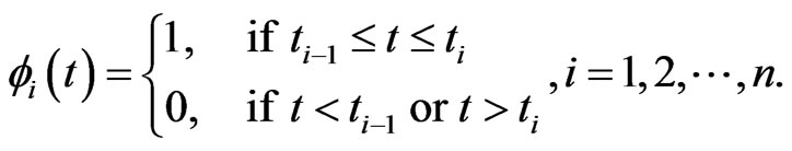
Using piecewise constant interpolating functions, we have
 (1.22)
 (1.23)
where  and
and  are the approximations for
  and
and , respectively, and
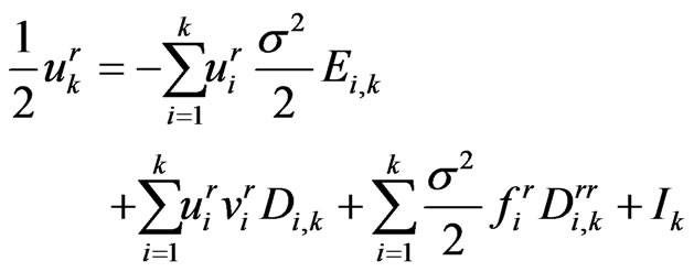
Substituting these approximations into the boundary integral Equation (1.20) at the collocation points, we have
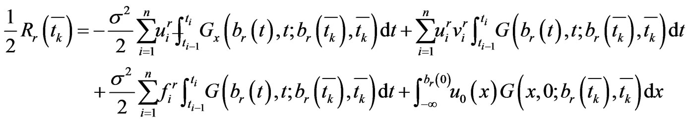 (1.24)
Let
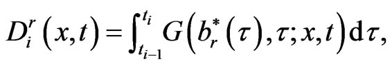 (1.25)
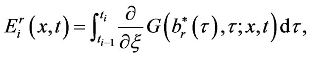 (1.26)
and
 (1.27)
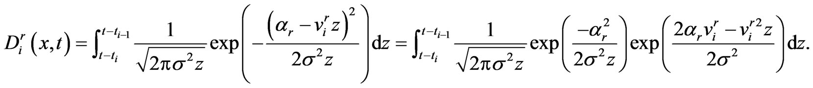
The quadrature rule for  can be derived as follows.
 (1.28)
Let  and
and , then
 (1.29)
Assuming  is small, the integral approximates
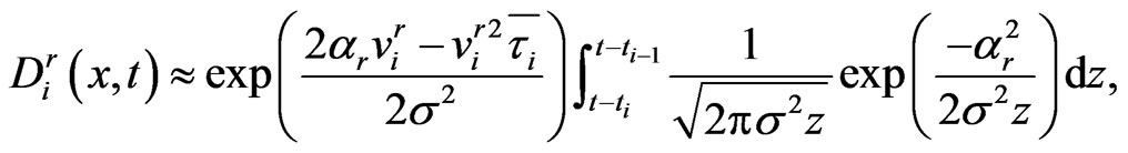 (1.30)
where . Let
. Let
 (1.31)
and
 (1.32)
Then we have the quadrature rule for ,
,
 (1.33)
where
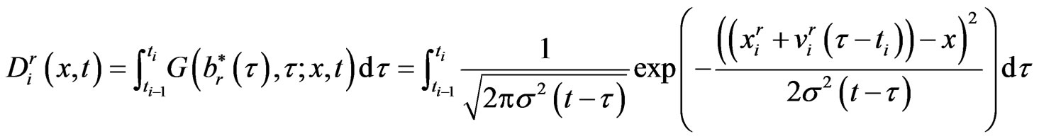
Similarly, quadrature rules for  is
is
 (1.34)
where
Simpson’s rule is used for the quadrature rule of integral . Let
. Let
 (1.35)
 (1.36)
 (1.37)
The boundary integral Equation (1.20) becomes
 (1.38)
and where  are the unknowns. It should be noted that
  and
and  are zeros when
 .
.
Rearranging Equation (1.38), we have
 (1.39)
Equation (1.39) is the stepping equation.
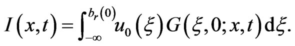
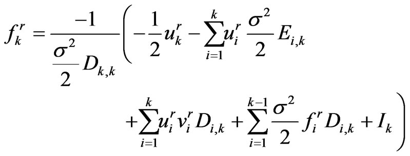
Therefore, we may solve  sequentially. By using the functions (1.25)-(1.27), the numerical solution of
  is
is
 (1.40)
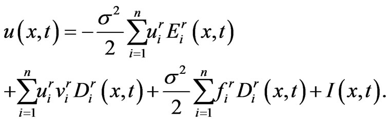
The option price  can be obtained by the inverse transformation,
 (1.41)
where .
.
5. A Numerical Example
In this section,a numerical example is presented to verify the boundary element formulation. We compute the prices of an option with a barrier. we consider a knock-out call. The barrier  is 100, i.e.
  is a constant with respect to time to maturity. The exercise price
  and rebate
  are 80 and 0 respectively. The volatility of underlying asset
  and risk free interest rate
  are 0.02 and 0.2 respectively. In this case, close form solution is available. Figure 1 shows the option price with respect to asset price. In this figure, time to maturity is 0.5. The exact prices are drawn with dashed line. The solid and dashed lines can not be distinct. Therefore we use Figure 2 to show the differences between the exact and numerical solutions. The differences are small.
6. Conclusion
In this article, Black Scholes’ equation and barrier condition are transformed to a boundary value problem of the heat equation. Then a bem is designed to solve this b.v.p.
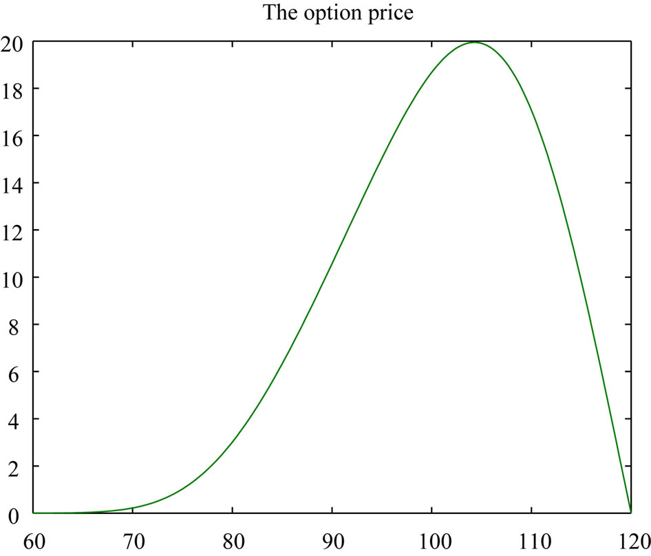
Figure 1. The numerical and exact solutions of . In this figure, time to maturity is 0.5. The exact solutions are drawn with dashed line, but the two curves coincide in this figure. Here
 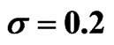 and
and  are used.
Figure 2. The differences between the exact and numerical solutions. The differences are small.
Finally, the method is applied to a barrier option. This formulation is correct.
REFERENCES
- F. Black and M. Scholes, “The Pricing of Options and Corporate Liabilities,” Journal of Political Economy, Vol. 81, No. 3, 1973, pp. 637-659. doi:10.1086/260062
- R. C. Merton, “Theory of Rational Option Pricing,” Bell Journal of Economics and Management Science, Vol. 4, No. 1, 1973, pp. 141-183. doi:10.2307/3003143
- J. C. Cox, S. A. Ross and M. Rubinstein, “Option Pricing: A Simplified Approach,” Journal of Financial Economics, Vol. 7, 1979, pp. 229-264. doi:10.1016/0304-405X(79)90015-1
- N. Kunitomo and M. Ikeda, “Pricing Options with Curved Boundaries,” Mathematical Finance, Vol. 2, No. 4, 1992, pp. 275-298. doi:10.1111/j.1467-9965.1992.tb00033.x
- H. Geman and M. Yor, “Pricing and Hedging DoubleBarrier Options: A Probabilistic Approach,” Mathematical Finance, Vol. 6, No. 4, 1996, pp. 365-378. doi:10.1111/j.1467-9965.1996.tb00122.x
- A. Pelsser, “Pricing Double Barrier Options Using Laplace Transforms,” Finance and Stochastics, Vol. 4, No. 1, 2000, pp. 95-104. doi:10.1007/s007800050005
- R. Zvan, K. R. Vetzal and P. A. Forsyth, “PDE Methods for Pricing Barrier Options,” Journal of Economics Dynamics & Control, Vol. 24, No. 11, 2000, pp. 1563-1590. doi:10.1016/S0165-1889(00)00002-6
- S. Sanfelici, “Galerkin Infinite Element Approximation for Pricing Barrier Options and Options with Discontinuous Payoff,” Decisions in Economics and Finance, Vol. 27, No. 2, 2004, pp. 125-151. doi:10.1007/s10203-004-0046-1
- A. M. L. Wang, Y. H. Liu and Y. L. Hsiao, “Barrier Option Pricing: A Hybrid Method Approach,” Quantitative Finance, Vol. 9, No. 3, 2009, pp. 341-352. doi:10.1080/14697680802595593
- S. Y. Shen and A. M. L. Wang, “On Stop-Loss Strategies for Stock Investments,” Applied Mathematics and Computation, Vol. 119, 2001, pp. 317-337. doi:10.1016/S0096-3003(99)00229-5