ABSTRACT

An explicit formula for the transition probability density function of the Hull and White stochastic volatility model in presence of nonzero correlation between the stochastic differentials of the Wiener processes on the right hand side of the model equations is presented. This formula gives the transition probability density function as a two dimensional integral of an explicitly known integrand. Previously an explicit formula for this probability density function was known only in the case of zero correlation. In the case of nonzero correlation from the formula for the transition probability density function we deduce formulae (expressed by integrals) for the price of European call and put options and closed form formulae (that do not involve integrals) for the moments of the asset price logarithm. These formulae are based on recent results on the Whittaker functions [1] and generalize similar formulae for the SABR and multiscale SABR models [2]. Using the option pricing formulae derived and the least squares method a calibration problem for the Hull and White model is formulated and solved numerically. The calibration problem uses as data a set of option prices. Experiments with real data are presented. The real data studied are those belonging to a time series of the USA S&P 500 index and of the prices of its European call and put options. The quality of the model and of the calibration procedure is established comparing the forecast option prices obtained using the calibrated model with the option prices actually observed in the financial market. The website: http://www.econ.univpm.it/recchioni/finance/w17 contains some auxiliary material including animations and interactive applications that helps the understanding of this paper. More general references to the work of the authors and of their coauthors in mathematical finance are available in the website: http://www.econ.univpm.it/recchioni/finance.

1. Introduction

We study the Hull and White stochastic volatility model [3] in presence of a (possibly) nonzero correlation between the stochastic differentials of the Wiener processes appearing on the right hand side of the model equations.

Let and be respectively the set of real and of positive real numbers and let t be a real variable that denotes time. The real stochastic processes, describe respectively the asset price and the associated stochastic variance as a function of time. The Hull and White stochastic volatility model assumes that , satisfy the following system of stochastic differential equations (see [3]):

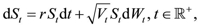(1)

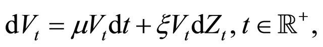(2)

where are real parameters. The processes, are standard Wiener processes such that, and, are their stochastic differentials. Moreover we assume that:

(3)

where denotes the expected value of ∙ and the quantity is a constant called correlation coefficient. The autocorrelation coefficients of the previous stochastic differentials are equal to one.

Equations (1) and (2) are equipped with the initial conditions:

(4)

(5)

where, are random variables that we assume to be concentrated in a point with probability one. For simplicity we identify the random variables, with the points where they are concentrated. We assume,. The assumption, with probability one and (1) and (2) imply that, with probability one for.

For later convenience we rewrite Equations (1) and (2) using the volatility process, , instead of the variance process,. Recall that we have:,. Equations (1) and (2) become:

(6)

(7)

where. Note that when and the Hull and White model (6), (7) reduces to the lognormal SABR model [4]. The lognormal SABR model is a generalization of the Black model in the context of stochastic volatility and is widely used in the practice of the financial markets.

Let us introduce the centered log-return , , and the quantity. Equations (6) and (7) can be rewritten as follows:

(8)

(9)

and the initial conditions (4) and (5) become:

(10)

(11)

where, are random variables that are concentrated in a point with probability one. Note that is concentrated in zero with probability one. Moreover the assumption that with probability one and (7) or (9) imply that with probability one for.

The Hull and White stochastic volatility models (1)-(5) has been introduced in mathematical finance in 1987 (see [3]) and is one of the first stochastic volatility models where a diffusion term that is time-varying and stochastic rather than being simply a constant is used to model the variance. More precisely in the Hull and White model a one factor model (i.e. Equation (2)) is used to model the variance (or the volatility) of the asset price (i.e. Equation (2) or (7)). When the transition probability density function of the Hull and White model and the corresponding European call and put option prices have been expressed with closed form formulae. In fact in [3] for the Hull and White model when it is shown that the price under a risk neutral measure at time t of a European call option with maturity time, such that, is given by the standard Black Scholes option pricing formula replacing the variance coefficient of the Black Scholes formula with an integrated average stochastic variance, , where

, , and taking the expected value of the resulting formula (see formula (8) in [3]). Note that in [3] no analytical expression for the probability distribution of the average stochastic variance, , is given. Only recently when a formula for the probability distribution of the average stochastic variance, , has been deduced [5]. Moreover in [5] when closed form formulae for European call and put option prices in the Hull and White model are given. Until now in the Hull and White model when the option prices have been computed using the Monte Carlo method (see [3,5-7]) or evaluating numerically series expansions in the correlation coefficient (see, for example, [8]).

In the last decade several modified versions of the Hull and White model have been proposed (see [8-11]). Some of these models contain a multifactor model of the asset price variance (or volatility). Usually in these models the characteristic function of the stochastic process implicitly defined by the model equations can be written explicitly (see, for example, [10,11] and the references therein). Models with nonzero correlation coefficients have been considered. However in these models the dependence of the asset price process from the “volatility process (or processes)” is substantially different than the dependence of these processes in the Hull and White model [3]. Generalizations of the Hull and White model (see, for example, [9]) in the context of jump diffusion models have also been considered. These generalizations usually retain the analytical treatability of the case of the Hull and White model.

In this paper when a formula for the transition probability density function associated to the processes, implicitly defined by (8)-(11) is deduced. This formula gives the transition probability density function of the stochastic processes, as a two dimensional integral of an explicitly known integrand and its deduction is based on some recent results on the Whittaker functions [1]. The formula obtained generalizes similar formulae deduced recently for the SABR and multiscale SABR models [2]. Thank to it when closed form formulae for the prices under a risk neutral measure of European call and put options in the Hull and White model and closed form formulae for the moments of, , and of, , are derived. The formulae of the European call and put option prices in the Hull and White model when are expressed as three dimensional integrals of explicitly known integrands. The closed form formulae for the moments of, , do not involve integrals and have been derived using a technique introduced in [12,13] in the study of the SABR model.

The moments of, , are also studied with the same technique, however for these last moments closed form formulae (that do not involve integrals) are available only for the moments of order smaller than two. The moments of, , of order greater or equal than two are expressed by formulae containing integrals of explicitly known integrands. Proceeding as done in [12,13] it is possible to use these moment formulae to study calibration problems for the Hull and White model when asset price data are considered.

In Section 3 proceeding as done in [14] we show that for the Hull and White model admits infinitely many risk neutral measures depending on a parameter. The risk neutral measures have the same expression of the physical measure when we interpret r as the risk-free interest rate and as a new drift that contains the risk premium parameter. This fact makes possible to deduce the option pricing formulae in a risk neutral context.

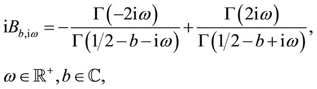
The results announced are based on the relation of the transition probability density function of the Hull and White model with the “heat kernel” of the index Whittaker transform [15]. The heat kernel of the index Whittaker transform, , is defined as follows:

(12)

where is the set of complex numbers, and i, sinh, , denote respectively the imaginary unit, the hyperbolic sine, the Whittaker function of indices (see [16] page 505) and the gamma function (see [16] page 253). Let and be the real part of b, in [17] it has been shown that a sufficient condition to guarantee the convergence for of the integral contained in (12) is,.

The kernel of the index Whittaker transform (12) generalizes the heat kernel of the Kontorovich-Lebedev transform [18,19] that has been used in [2] to derive the explicit formulae of the transition probability density functions of the normal and lognormal SABR and multiscale SABR models.

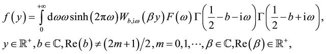
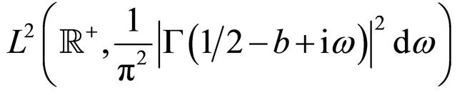
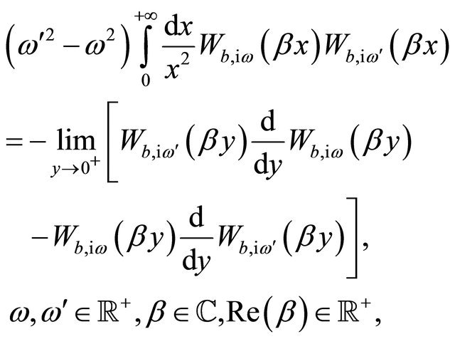
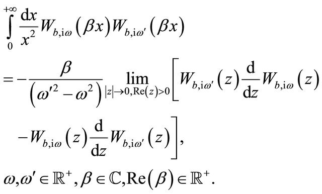
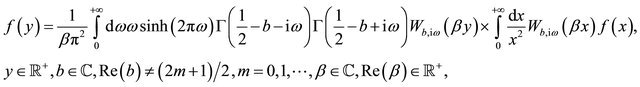
Let be the Hilbert space of the functions defined on that are Lebesgue square integrable in with respect to the measure. In our analysis of the Hull and White model we deduce the following formula (see Appendix A):

(13)

Note that the integrals contained in formula (13) must be interpreted in the sense of distributions. Formula (13) is a straightforward consequence of the result presented in [1] and generalizes the inversion formula for the Macdonald transform presented in [20] and used in [2]. In [1] no restrictions on b are considered. Note that the condition is a sufficient condition to guarantee the regularity of the functions, , , (see [17] for further details) that appear in (13).

Finally using the option pricing formulae deduced a calibration problem for the Hull and White model (1), (2) is formulated as a nonlinear constrained least squares problem and is solved numerically. The calibration problem considered uses as data a set of option prices. Given the asset prices the calibrated model is used to forecast option prices. Numerical experiments with real data are presented. The real data studied are those belonging to a time series of the USA S&P 500 index and of the prices of its European call and put options. In particular forecast option prices obtained using the calibrated model are compared with the option prices actually observed in the financial market. This comparison establishes the quality of the model and of the calibration procedure.

The website: http://www.econ.univpm.it/recchioni/finance/w17 contains some auxiliary material including animations and interactive applications that helps the understanding of this paper. A more general reference to the work of the authors and of their coauthors in mathematical finance is the website: http://www.econ.univpm. it/recchioni/finance.

The remainder of the paper is organized as follows. In Section 2 when we derive a formula for the transition probability density function of. In Section 3 we deduce a closed form expression for the first two moments of, , and an integral representation formula for the higher moments of,. In Section 4 we derive a recursive formula for the moments of,. This recursive formula is used to obtain closed form expressions of the first three moments of,. In Section 5 we derive formulae for the option prices in the Hull and White model. The formulae deduced in Sections 2-5 hold when. In Section 6 using the previous option pricing formulae we formulate a calibration problem for the Hull and White model. Moreover we present a forecasting procedure that, given the asset price at the time of the forecast, forecasts option prices using the calibrated model. The calibration problem and the forecasting procedure are tested in numerical experiments with real data. The real data studied are those belonging to a time series of the USA S&P 500 index and of its European option prices. Finally Section 7 is made of two Appendices that contain some auxiliary formulae used in the paper.

2. The Transition Probability Density Function

Let us consider the Hull and White models (8)-(11). We denote with, , , , , the transition probability density function of the stochastic processes, , implicitly defined by (8)-(11). The function is the probability density function of having, given the fact that, , when, , , and. When we must choose,. Note that the backward Kolmogorov equation associated to (8), (9) is invariant by time translation and that this implies that p is a function of instead of being a function of t and separately when,. We denote with, , , the function considered as a function of the variables. The function, , , satisfies the backward Kolmogorov equation associated to (8), (9):

(14)

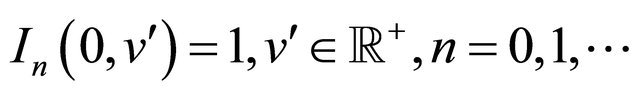
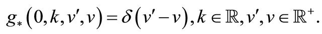
and the initial condition:

(15)

where denotes the Dirac’s delta. Recall that is defined as follows:

(16)

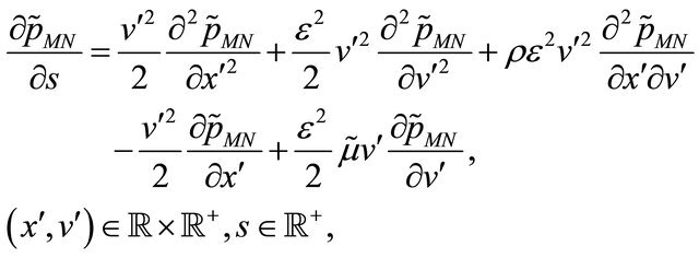
We show that:

(17)

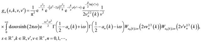
where g is given by:

(18)

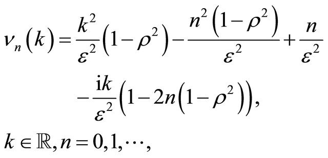
The functions ν(k) and a(k), , in (18) are given by:

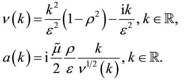(19)

Formulae (16), (18) and (19) hold when.

Note that when and formula (18) contains the heat kernel of the index Whittaker transform (12) and that when formula (18) can be rewritten as follows:

(20)

where, is the modified Bessel function of the second kind with purely imaginary index (see [16] page 375). Moreover when substituting (20) in (17) we have:

(21)

where:

(22)

Formulae (17), (18) and (21), (22) are the main results of this section.

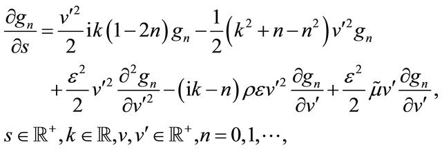
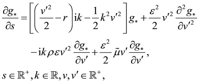
Let us derive formula (18). Substituting (17) in (14), (15) it is easy to see that if the function g satisfies the initial value problem:

(23)

(24)

Equations (14) and (15) hold. Note that the initial value problem (23), (24) depends on the parameter and recall that k is the conjugate variable in the Fourier transform of the variable.

Let us seek the solution of problem (23), (24) in the following form:

(25)

where L is a function that must be determined and (the constant) will be chosen later. Substituting (25) in (23) it is easy to see that (23) holds if L as a function of satisfies the following equation:

(26)

where and, are given by (16), (19) respectively. To solve (26) let us make the following change of dependent variable:

(27)

Moreover in (26) let us consider the new dependent variable Q as a function of the new independent variable. Note that the variable z is considered as a complex variable. Let be the function Q as a function of. Choosing from (26), (27) it follows that satisfies the equation:

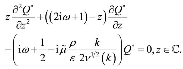(28)

Equation (28) is known as Kummer’s equation (see [16] page 504). The solution of (28) that decays exponentially when is (see [21] page 797):

(29)

where is a constant with respect to that must be determined in order to satisfy the initial condition (24) and, is defined in (19).

Substituting (29) and (27) in (25) we obtain:

(30)

To impose the initial condition (24) we use formula (24)) (see Appendix A) from which we obtain the following expression for:

(31)

Substituting (31) in (30) we obtain formula (18).

When formula (20) can be deduced from formula (18). In fact when we have, , and the following relations hold (see F. Oberhettinger [22] page 287 and [16] page 256, formula 6.1.30):

(32)

(33)

Finally formulae (21), (22) that hold when are obtained rewriting the expression (20) of g when using (32), (33), the formula for the Laplace transform of the function, , (see [23], page 146 formula (26)), that follows:

(34)

and the representation formulae:

(35)

(36)

Formulae (35) and (36) can be deduced from formula (46) page 35 of [23], formula (9) page 176 of [24], and formula (1.1) of [20] (see [2] for further details).

Note that the technique used here to obtain formulae (17), (18) and (21), (22) is similar to the one used in [2] to deduce the formula for the transition probability density function of the lognormal SABR model.

3. Moments of the Asset Price

Let, and be the moment with respect to zero of the variable, implicitly defined by (1)-(5), that is:

(37)

where is given by (17) and we have and.

Let us rewrite formula (17) as follows:

(38)

where the functions, will be determined later in this section. Using (38) Equation (37) becomes:

(39)

where, , ,

. That is for the knowledge of the n-th moment of the state variable, is reduced to the knowledge of. To determine we derive an initial value problem for a partial differential equation satisfied by,. Note that when the function is the function g given by (18) and that the partial differential equation satisfied by that we are looking for is Equation (23).

Substituting (38) in (14), (15) it is easy to see that the functions, , satisfy the following partial differential equations:

(40)

with initial conditions:

(41)

Proceedings as done in Section 2 when n = 0 to solve problem (23), (24) it is easy to see that the solution of (40), (41) that guarantees that is a probability density function is:

(42)

where the functions and, , are defined as follows:

(43)

(44)

For when the function g_n (i.e. the function) satisfies problem (40), (41) with k = 0. Integrating with respect to v when Equations (40), (41) when k = 0, we obtain a set of initial value problems satisfied by the functions,. That is we obtain the following partial differential equations:

(45)

with initial condition:

(46)

It is easy to see that when the solution of problem (45), (46) is. From (39) it follows that:

(47)

When problem (45), (46) can be solved using (42) and we have:

(48)

Substituting formula (48) in equation (39) we obtain the integral representation formula for the moments, , announced in the Introduction.

For in order to guarantee that the function does not diverge when v goes to plus infinity and that is well defined we must require that the real part of is positive (i.e.). This implies that the following condition holds:

(49)

Condition (49) can be rewritten as a condition for given, that is:

(50)

For condition (50) guarantees the convergence on the n-th moment of,. The same condition for the convergence of the n-th moment of, , in the case of negative correlation (i.e. the condition) has been derived in a different way in the study of the lognormal SABR model (i.e. the model obtained choosing, in (6), (7)) in [25] Theorem 2.3. Note that condition (49) for the convergence of the n-th moment can be rewritten as a condition for n given, in this case we have:

(51)

From the formula, , , , and from Equations (6) and (7) it follows that a risk neutral measure of the Hull and White model has the same expression of the physical measure when r is substituted with the risk free interest rate and is replaced with where where is the risk premium parameter (see [14] Theorem 4.1 and [26], pp. 17-18). That is there are infinitely many risk neutral measures in the Hull and White model depending from the value of the risk premium parameter.

This last observation allows us to interpret the formulae derived in Section 5 to price European call and put options under the physical measure as formulae to price these options under a risk neutral measure. Note that calibrating the Hull and White model (1), (2) using asset prices as data we can estimate the parameters of the physical measure and consequently the parameters, and that calibrating the Hull and White model (1), (2) using option prices as data we can estimate the risk neutral parameters,. Recall that cannot be observed in the financial markets and that can be considered as a parameter that must be determined in the calibration procedure. The values of the parameters and obtained in this way determine the value of the risk premium parameter.

4. Moments of the Logarithm of the Asset Price

The processes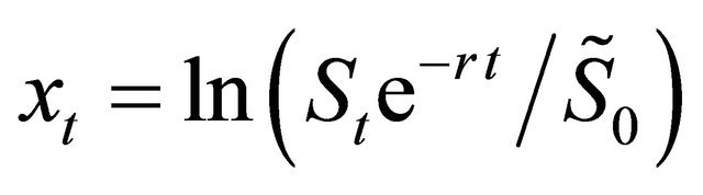, , , satisfy Equations (8)-(11) and as a consequence the processes, , , satisfy the equations:

(52)

(53)

the initial conditions:

(54)

(55)

and the assumption (3) on the correlation of the stochastic differentials.

For let, be the moment with respect to zero of, , we have:

(56)

where is the transition probability density function associated to the stochastic processes, implicitly defined by (52)-(55). The function can be written as follows:

(57)

and the function can be determined proceeding as done in Section 2. Note that depends on and not on and separately, , so that we can rewrite the moments of, defined in (56) as follows:

(58)

where

(59)

Proceeding as done in [12,13] in the study of the normal and lognormal SABR models and in Section 3 to deduce the initial value problems (40), (41) and (45), (46) satisfied by the functions, it is possible to write an initial value problem satisfied by the function and to deduce from it initial value problems satisfied by the functions That is it can be shown that, , satisfies the following problem:

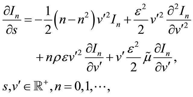
(60)

with the initial condition:

(61)

and that the functions, satisfy the problems:

(62)

with the initial conditions:

(63)

Note that in (62) when we set .

It is easy to see that the solution of problem (60), (61) is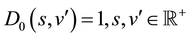. In order to solve the initial value problems (62), (63) let us consider the following change of (independent) variable, , and let be the function expressed in the new variable, that is let, , ,. The solutions, of the problems (62), (63) expressed in the variables, are given by:

(64)

where

(65)

The integral in the variable in (64) is an elementary integral that can be computed using the following formula:

(66)

Formulae (64)-(66) together with some elementary computations give:

(67)

(68)

Let us choose, we have in (58), (67) and (68). It follows that and that the first three moments of, are given by:

(69)

(70)

(71)

Proceeding as done to deduce (67)-(71) the expressions of the functions, , , and of the moments, , , , for can be obtained. These expressions become more and more involved when n increases. Note that formulae (70) and (71) are closed form formulae containing only elementary functions of quantities that can be observed in the financial markets. These formulae can be used to formulate calibration problems for the Hull and White model. Thank to the closed form character of these formulae it is possible to develop very efficient numerical algorithms to solve these calibration problems. In [12, 13] this idea has been exploited to calibrate the normal and the lognormal SABR models.

5. Option Pricing Formulae

Let us derive in the Hull and White model the formulae of the prices at time of European call and put options having maturity and strike price. These formulae express the option prices as three dimensional integrals of explicitly known integrands.

To this aim we rewrite the transition probability density function (17) as follows:

(72)

where c is a constant and g_c is a function to be determined. Let us derive the expression of the function g_c. Substituting (72) in (14), (15) it is easy to see that if g_c satisfies the following partial differential equation:

(73)

with the initial condition:

(74)

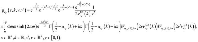
the Equations (14) and (15) hold. Recall that. Proceeding as done in Section 2 we deduce the following formula:

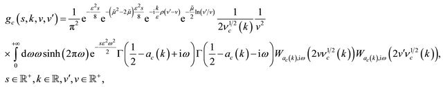(75)

where the functions, are given by:

(76)

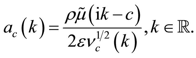(77)

Note that in order to guarantee that for the function does not diverge when v goes to plus infinity and that the function, , is well defined we must require that for the real part of is positive. An easy computation shows that the condition, implies that c must satisfy the following inequalities:

(78)

or

(79)

Let us choose c as follows:

(80)

Note that the choice of c made in (80) when satisfies conditions (78) and (79), that is (80) is a satisfactory choice of c for. We rewrite the transition probability density function as follows:

(81)

where the function that appears in (81) is given by:

(82)

and the functions, are given by:

(83)

(84)

The price at time of a European call option having maturity and strike price is the expected value of the discounted payoff with respect a risk neutral measure. As shown in Section 3 the risk neutral measures of the Hull and White model are obtained replacing in the physical measure the parameter r with the risk free interest rate and the parameter with where is the risk premium parameter. That is we have:

(85)

where is the asset price at time t = 0 and is the maximum between ∙ and zero and p is a risk neutral transition probability density function. That is in (85) the function p is given by (81) with the parameters r^* and instead of r and respectively. Note that the initial stochastic volatility is not observable and must be determined in the calibration process.

Using formulae (81) and (85) we have:

(86)

In (86) the integral in the variable x can be computed explicitly, in this way formula (86) can be reduced to the following formula:

(87)

where is given by (82), and in (82) and replace r and respectively. Note that on the right hand side of (86), (87), we have, however the prices on the left hand side of (86), (87) do not depend on. In the numerical experiments presented in Section 6 we choose.

The price at time of a European put option having maturity and strike price can be obtained using the put call parity relation. That is using the relation:

(88)

where in the transition probability density p the parameters, replace r, respectively. Formula (88) follows immediately from the fact that the option prices are the expected value of the discounted payoffs with respect to a risk neutral measure. From (88) and the formulae for the first two moments of, , contained in (47) we have:

(89)

6. Calibration Problem and Numerical Experiments

Let us consider option prices under a risk neutral measure. That is let us substitute the models (52)-(55) with the model:

(90)

(91)

together with the initial conditions:

(92)

(93)

where, are standard Wiener processes such that, and, are their stochastic differentials. The correlation structure of the model is assumed to be:

(94)

where.

The models (90)-(93), (92) is parameterized by five real parameters, that is:.

Let be the five-dimensional real Euclidean space, let us introduce the vector given by and the set defined as follows:

(95)

The inequalities that define are dictated by the “meaning” of the parameters in the model equations. In the calibration problem that we study the vector is the unknown that must be determined from the data and is the set of the “feasible” choices of. We use as data of the calibration problem a set of option prices observed at a given time and we formulate the calibration problem as a nonlinear constrained least squares problem. This means that solving the calibration problem consists in fitting in the least squares sense, under the constraints defined in (95), the observed option prices (i.e. the data) with the option prices obtained evaluating the formulae deduced in Section 5 adapted to the circumstances.

Let be positive integers, be the observation time and be the asset price observed at time

. Let, ,

, , be respectively the observed prices at time of the European call options having maturity time and strike price, , and of the European put options having maturity time and strike price,. Note that the values, , , and, , , are not necessarily distinct. For example prices of options having the same maturity time and several strike prices can be considered as data, in this case in the previous sets of values some of the maturity times are repeated. Of course we assume, , and,.

Let and let,

, , , be the prices as a function of at time of the European call and put options obtained evaluating, respectively, formulae (87) and (88). Some obvious transformations of the data and of the formulae are necessary to evaluate the option prices using formulae (87) and (88). In fact, for example, in (87) and (88) we have chosen instead of leaving as a generic time value as done in this Section where we study real data.

The numerical quadratures necessary to evaluate (87) and (88) are done using the composite midpoint quadrature rule with 200 nodes in the k coordinate and 10 nodes in the v and coordinates. This choice guarantees approximately three significant digits to be correct in the option prices computed in the numerical experiments presented here. With these choices of the discretization parameters one evaluation of formula (87) requires approximately 40 seconds on the Intel CORE Duo CPU T6400 2 GHz processor. However it must be pointed out that the evaluation of several options (i.e. for example of a few dozens of options) that differ only for the value of the strike price requires approximately the same time than the evaluation of a single option when the computation is implemented exploiting the properties of the option pricing formulae. The calibration problem considered is formulated as follows:

(96)

where the objective function is given by:

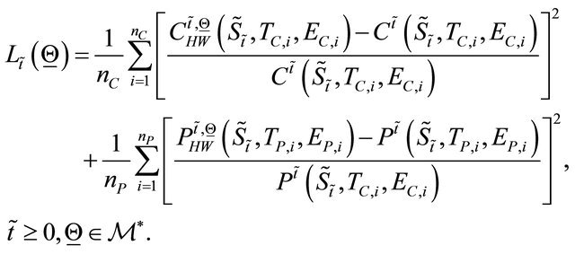(97)

The nonlinear constrained least squares problem (96) is only one possible formulation of the calibration problem studied between many other possible formulations.

In the numerical experiment that follows we solve problem (96) with a local minimization method. We choose the initial guess of the minimization procedure used to solve problem (96) exploring the feasible region. This is done taking a set of random points belonging to and evaluating the objective function on this set of points. The initial guess of the minimization method is chosen among these random points using a heuristic rule. The minimization method used is a variable metric steepest descent method (see [27]). This method is an iterative procedure that, given an initial vector, generates a sequence, , of vectors such that, , and,. For the vector is obtained from the vector making a step of appropriate length in the direction of minus the gradient with respect to of computed in a suitable metric that depends on the constraints defined in. The procedure stops when the following criterion is satisfied:

(98)

where, are given positive constants. Details about the variable metric steepest descent method used to solve the calibration problem can be found in [28].

In the numerical experiment presented here we consider the closing value of the day of the USA S&P 500 index and the closing prices of the day of the European call and put options on the USA S&P 500 index with expiry date March 16th, 2013 and strike prices , , . These prices are observed in the time period that goes from April 2nd, 2012, to July 25th, 2012. Note that the observations are daily observations. Recall that in the study of financial data time series a year is made of about 252 trading days and a month is made of about 21 trading days. Figure 1 shows the value of the USA S&P 500 index as a function of time during the period of interest. Figures 2 and 3 show respectively the prices of the European call and put options on the index with maturity time March 16th, 2013 and strike price, , specified previously as a function of time during the same time period.

Let, , , we have that. We calibrate the Hull and White models (90)-(93) every (trading) day during the period that goes from to using the prices of the European call and put options shown in Figures 2 and 3 when. That is we consider a rolling window made of the data of a day that covers the period April 2nd, 2012, May 15th, 2012 (thirty trading days) and we solve the corresponding thirty calibration problems (96) with, , ,. The calibration procedure stops according to criterion (98) where we have chosen,.

Figure 4 shows the risk neutral parameters obtained using the calibration procedure. We can see that the parameter values as functions of time do not change significantly. That is the values of the parameters of the models (90)-(93) obtained solving the calibration problem are somehow “stable” during the observation period. The values of the parameters shown in Figure 4 are used to forecast the option prices one day ahead. That is we use the parameter values obtained calibrating the model with the data of to compute the option prices at, obtained using,. The forecasts of the option prices are obtained evaluating the European call option with formula (87) and the European put option with the put call parity relation (89) given the call price. Of course the formulae (87) and (89) must be adapted, with some obvious changes, to take care of the circumstances of the data time series. Figure 5 shows the observed and forecast values of the European call and put option prices. The average relative errors on the forecast values of the European call and put option prices when compared with the corresponding prices observed in the financial market are respectively 8% and 5% Note that if we remove from the constraint contained in the definition of the request that must be non negative the solution of the calibration procedure shows a negative risk free interest rate of about minus 2% (see Figure 6) with an average of the relative errors between forecast and observed call and put prices respectively of approximately 2% and 3% (see Figure 7 and http://www. econ.univpm.it/recchion/finance/w17). That is if we allow negative risk free interest rates we improve the forecast of the prices of the European call and put options. This unexpected finding may be a consequence of the anomalous market conditions registered in the spring 2012.

Finally we observe that the initial stochastic volatility

does not show significant changes during the period April 2nd, 2012, May 15th, 2012. This is a plausible result when compared to the behaviour of the USA S&P 500 VIX index (SOURCE MKT 500 Currency USD) shown in Figure 8. In fact the USA S&P 500 VIX index monitors the volatility of the USA S&P 500 index and we can see in Figure 8 that in the period April 2nd, 2012, May 15th, 2012 the USA S&P 500 VIX index remains substantially unchanged.

REFERENCES

Appendices

Appendix A

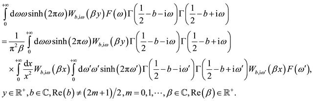
In this Appendix we derive formula (31). To this aim we first prove the following formula:

(99)

that generalizes the already known formula (see [1] Section 1, formula (1.2)):

(100)

We interpret the integrals contained in formulae (99), (100) in the sense of distributions. As mentioned in [17] the constant b is restricted by the condition

, , in order to avoid the singularities of the functions and

, that occur when the arguments of the Gamma functions are equal to zero or to a negative integer (see [17] for further details).

We prove (99) arguing as done in [1]. Let us recall that the functions, satisfy the following differential equations:

(101)

(102)

Equations (101), (102) follow immediately from of the Whittaker equation (see [16] p. 505 formula 13.1.31) that defines the Whittaker functions. Multiplying Equations (101), (102) respectively by and by , subtracting the resulting equations one from the other and integrating with respect to x when and, we obtain:

(103)

Taking into account that, , , (see [16] p. 504 formula 13.1.8 and p. 505 formulae 13.1.32, 13.1.34, 13.1.34, and [1] for further details), and integrating by part (103) we obtain:

(104)

where means the right-handed limit in zero of the function. Let, Equation (104) can be rewritten as follows:

(105)

Let us recall that the asymptotic behaviour when and of, (see [1] formula (2.5), [16] p. 504 formula 13.1.2, p. 505 formulae 13.1.32, 13.1.34) is:

(106)

where

(107)

(108)

and is the Landau symbol. Evaluating the limit on the right-hand side of (105) as done in [1] Section 3 and using formulae (106)-(108), we obtain:

(109)

Formula (109) reduces to formula (99), in fact we have:

(110)

Let us prove now formula (31). We use formula (99) and the following integral transform:

(111)

that maps the function, , into the function,. The integral appearing in (111) must be interpreted in the sense of distributions. When the integral transform (111) reduces to the transform studied in [15]. This last transform is called index Whittaker transform. Note that in [15] it is shown that for

when b is real and the integral operator appearing in (111) maps

in.

Using (99) it is easy to see that the following equation holds:

(112)

when, , belongs to a suitable class of distributions. The characterization of this class of distributions goes beyond the purposes of this paper and is omitted.

Multiplying Equation (112) by

and integrating with respect to when we obtain:

(113)

Using definition (111) on both sides of Equation (113) we obtain the following identity:

(114)

that holds when, belongs to a suitable class of distributions. Equation (114) reduces to Equation (13) when.

Note that in order to determine the constant in formula (31) we must use formula (114) when is the Dirac’s delta, that is we must use the following formula:

(115)

Appendix B

In this Appendix we give some details about the derivation of formulae (60), (61) and (62), (63). Let us recall that formula (59) defines, , ,.

It is easy to see that the function of (57) satisfies the equation:

(116)

with the initial condition:

(117)

For, let ,.

Using Equations (116), (117) when we have that satisfies the equation:

(118)

with the initial condition:

(119)

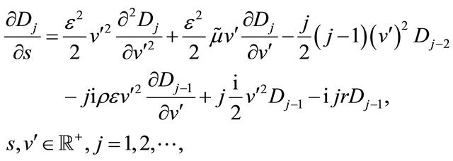
For the equations satisfied by are obtained deriving j times with respect to k Equations (116), (117) and setting in the resulting equations. We have:

(120)

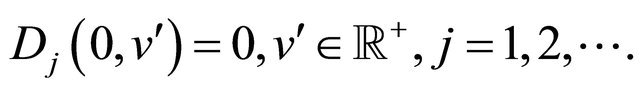
with the initial condition:

(121)

where we define.

Integrating with respect to v when Equations (118), (119) and (120), (121) we obtain respectively Equations (60), (61) and (62), (63).

REFERENCES

- R. Szmytkowki and S. Bielski, “An Orthogonality Relation for the Whittaker Functions of the Second Kind of Imaginary Order,” Integral Transforms and Special Functions, Vol. 21, No. 10, 2010, pp. 739-744. doi:10.1080/10652461003643412
- L. Fatone F. Mariani, M. C. Recchioni and F. Zirilli, “Some Explicitly Solvable SABR and Multiscale SABR Models: Option Pricing and Calibration,” Journal of Mathematical Finance, Vol. 3, No. 1, 2013, pp. 10-32.
- J. Hull and A. White, “The Pricing of Options on Assets with Stochastic Volatilities,” The Journal of Finance, Vol. 42, No. 2, 1987, pp. 281-300. doi:10.1111/j.1540-6261.1987.tb02568.x
- P. S. Hagan, D. Kumar, A. S. Lesniewski and D. E. Woodward, “Managing Smile Risk,” Wilmott Magazine, 2002, pp. 84-108. http://www.wilmott.com/pdfs/021118-smile.pdf
- C. O. Ewald, K. R. Schenk-Hoppé and Z. Yang, “ClosedForm Solutions for European and Digital Calls in the Hull and White Stochastic Volatility Model and Their Relation to Locally R-Minimizing and Delta Hedges,” Paper No. 07-11, Swiss Finance Institute Research, 2007. http://papers.ssrn.com/sol3/papers.cfm?abstract-id=957807
- C. Corrado and T. Su, “Empirical Test of the Hull and White Option Pricing Model,” The Journal of Futures Markets, Vol. 18, No. 4, 1998, pp. 363-378. doi:10.1002/(SICI)1096-9934(199806)18:4<363::AID-FUT1>3.0.CO;2-K
- B. A. Surya, “Two-Dimensional Hull-White Model for Stochastic Volatility and Its Nonlinear Filtering Estimation,” Procedia Computer Science, Vol. 4, 2011, pp. 1431- 1440. doi:10.1016/j.procs.2011.04.154
- E. Alòs, “A Generalization of the Hull and White Formula with Applications to Option Pricing Approximation,” Finance and Stochastics, Vol. 10, No. 3, 2006, pp. 353-365. doi:10.1007/s00780-006-0013-5
- E. Alòs, J. A. León, M. Pontier and J. Vives, “A Hull and White Formula for a General Stochastic Volatility Jump- Diffusion Model with Applications to the Study of the Short-Time Behavior of the Implied Volatility,” Journal of Applied Mathematics and Stochastic Analysis, 2008, Article ID: 359142, 17 p.
- L. A. Grzelakab, L. A. Oosterleeac and S. Van Weeren, “Extension of Stochastic Volatility Equity Models with the Hull-White Interest Rate Process,” Quantitative Finance, Vol. 12, No. 1, 2012, pp. 89-105. doi:10.1080/14697680903170809
- E. Benhamou, E. Gobet and M. Miri, “Analytical Formulas for a Local Volatility Model with Stochastic Rates,” Quantitative Finance, Vol. 12, No. 2, 2012, pp. 185-198. doi:10.1080/14697688.2010.523011
- L. Fatone, F. Mariani, M. C. Recchioni and F. Zirilli, “The Use of Statistical Tests to Calibrate the Normal Sabr Model,” Journal of Inverse and III Posed Problems, Vol. 21, No. 1, 2013, pp. 59-84.
- L. Fatone, F. Mariani, M. C. Recchioni and F. Zirilli, “Closed Form Formulae for the Moments of the Lognormal SABR Model Variables and Their Use to Solve Two Calibration Problems,” Inverse Problems in Science and Engineering, 2012.
- B. Wong and C. C. Heyde, “On Changes of Measure in Stochastic Volatility Models,” Journal of Applied Mathematics and Stochastic Analysis, 2006, Article ID: 18130, 13 p. doi:10.1155/JAMSA/2006/18130
- S. B. Yakubovich and M. M. Rodrigues, “Heat Kernel in Terms of Whittaker’s Functions,” International Symposium on Orthogonal Polynomials and Special Functions—A Complex Analytic Perspective, Copenhagen, 11- 15 June 2012. http://cmup.fc.up.pt/cmup/v2/include/filedb.php?id=398&table=publicacoes&field=file
- M. Abramowitz and I. A. Stegun, “Handbook of Mathematical Functions,” Dover, New York, 1970.
- P. A. Becker, “On the Integration of Products of Whittaker Functions with Respect to the Second Index,” Journal of Mathematical Physics, Vol. 45, No. 2, 2004, pp. 761-773. doi:10.1063/1.1634351
- S. B. Yakubovich, “The Heat Kernel and Heisenberg Inequalities Related to the Kontorovich-Lebedev Transform,” Communications on Pure and Applied Analysis, Vol. 10, No. 2, 2011, pp. 745-760. doi:10.3934/cpaa.2011.10.745
- S. B. Yakubovich, “Beurling’s Theorems and Inversion Formulas for Certain Index Transforms,” Opuscula Mathematica, Vol. 29, No. 1, 2009, pp. 93-110.
- R. Szmytkowki and S. Bielski, “Comment on the Orthogonality of the Macdonald Functions of Imaginary Order,” Journal of Mathematical Analysis and Applications, Vol. 365, No. 1, 2010, pp. 195-197. doi:10.1016/j.jmaa.2009.10.035
- R. Beals and Y. Kannai, “Inverse Laplace Transforms of Products of Whittaker Functions,” Proceedings of the Royal Society A, Vol. 464, No. 2092, 2008, pp. 795-806. doi:10.1098/rspa.2007.0248
- F. Oberhettinger, “Tables of Bessel Transform,” Springer-Verlag, Berlin, 1972. doi:10.1007/978-3-642-65462-6
- A. Erdelyi, W. Magnus, F. Oberhettinger and F. G. Tricomi, “Tables of Integral Transforms,” McGraw-Hill Book Company, New York, 1954.
- P. L. Lions and M. Musiela, “Correlation and Bounds for Stochastic Volatility Models,” Annales de l’Institut Henri Poincare (C) Non Linear Analysis, Vol. 24, No. 1, 2007, pp. 1-16.
- W. Schoutens, “Lévy Processes in Finance,” John Wiley & Sons, Chichester, 2003. doi:10.1002/0470870230
- A. Mordecai, “Nonlinear Programming: Analysis and Me-thods,” Dover Publishing, New York, 2003.
- L. Fatone, F. Mariani, M. C. Recchioni and F. Zirilli, “An Explicitly Solvable Multi-Scale Stochastic Volatility Model: Option Pricing and Calibration,” The Journal of Futures Markets, Vol. 29, No. 9, 2009, pp. 862-893. doi:10.1002/fut.20390