Applied Mathematics
Vol.4 No.1(2013), Article ID:27090,5 pages DOI:10.4236/am.2013.41003
A Modified Homotopy Analysis Method for Solving Boundary Layer Equations
School of Naval Architecture, Ocean and Civil Engineering, Shanghai Jiao Tong University, Shanghai, China
Email: zhaoyl@sjtu.edu.cn
Received October 28, 2012; revised November 28, 2012; accepted December 4, 2012
Keywords: Homotopy Analysis Method; Boundary Layer Equations; Orthonormal Functions
ABSTRACT
A new modification of the Homotopy Analysis Method (HAM) is presented for highly nonlinear ODEs on a semi-infinite domain. The main advantage of the modified HAM is that the number of terms in the series solution can be greatly reduced; meanwhile the accuracy of the solution can be well retained. In this way, much less CPU is needed. Two typical examples are used to illustrate the efficiency of the proposed approach.
1. Introduction
In 1992, Liao [1] proposed the Homotopy Analysis Method (HAM) to solve nonlinear differential equations analytically. Since then, HAM has been used to investigate a variety of mathematical and physical problems [2]. As is well known, HAM has the advantage of independence on small physical parameters and adjusting the convergence region and convergence rate of the series solution over perturbation method. However, for some type of auxiliary operator (i.e. base functions), it is usually time-consuming to get high-order approximation, and the number of terms appearing in high order approximation is very huge.
To improve the efficiency of HAM, many scholars have proposed different techniques. Yabushita [3] suggested an optimal HAM approach by minimizing the residual of governing equations. Marinca [4], Niu [5], Liao [6] developed this kind of approach. Lin [7] suggested an iterative technique, in which the initial guess is continuously replaced by intermediate approximation to proceed the computation. Recently, we use orthonormal polynomials/ functions to approximate the right-hand side of the highorder deformation equations to prohibit the rapid growth of the terms appearing in approximate solutions. For differential equations defined on a finite interval, trigonometric functions (or polynomial functions) are usually selected to express solutions. In this case, orthonormal trigonometric functions (or Chebyshev polynomials) are used to approximate right-hand side of high-order deformation equations. In this paper, we generalize this kind of approach for nonlinear problems defined on semi-infinite intervals. The main idea is that orthonormal functions derived from Schmidt-Gram process are used to approximate the right-hand side of high-order deformation equations during computation. For different types of problems, the derived orthonormal functions are different, which are closely related to the solution expression.
In the following section, the modified HAM (MHAM) is presented for boundary layer problems. In Section 3, examples are given to demonstrate it. Conclusions and some discussions are given in the last section.
2. Analysis of the Method
For convenience, a brief description of the standard HAM will be present first. Then the proposed truncation technique will be followed.
Without loss of generality, consider the differential equation
 , (1)
, (1)
where N is a nonlinear operator, t denotes the independent variable,  is an unknown function. Suppose
  could be expressed by a set of functions
 (2)
(2)
such that
 (3)
(3)
is uniformly valid, where  is a coefficient. In HAM, the zeroth-order deformation equation is constructed as
 , (4)
, (4)
where
 , (5)
, (5)
![]() is an auxiliary linear operator, and
is an auxiliary linear operator, and  the auxiliary function. Applying the homotopy-derivative [8]
 (6)
(6)
to both sides of Equation (4), we get the corresponding mth-order deformation equation
 , (7)
, (7)
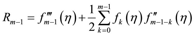
where
 , (8)
, (8)
and
 (9)
(9)
Note that  can be obtained by solving linear Equation (7) one after the other. The mth-order approximation of
  is given by
 (10)
(10)
To measure the accuracy of , the squared residual error for Equation (1) is defined as
 where
where  is the domain.
If a successful homotopy analysis solution is obtained, the difficulty to get better approximation is that with the growth of order, the number of terms in higher-order approximation will grow rapidly, resulting in an enormous amount of computing time. To address this problem, we propose a truncation technique. The basic idea is that the right-hand side of Equation (7) is approximated by a set of orthonormal functions.
Suppose that  can be expressed by a finite linear combination of linearly independent functions
 ,
, . Note that
  may be slightly different from
 . Define a proper inner product in the linear space spanned by
  as
as
 , (11)
where  is a weight function. In the framework of HAM, two typical kinds of base functions are usually used for boundary layer problems.
Case 1: suppose that  can be expressed by finite linear combination of linearly independent functions
 (12)
(12)
Note that (12) is dependent on three parameters![]() , m and n. To implement the orthonormalization, an order is given to (12) as follows (called triangular order):
, m and n. To implement the orthonormalization, an order is given to (12) as follows (called triangular order):
 .
.
The inner product is defined as

Case 2: suppose that  can be expressed by finite linear combination of linearly independent functions
 . (13)
The inner product is defined as
 . (14)
Applying the Schmidt-Gram process to the first  functions
 ,
, ,
, ,
,  , we obtain
  orthonormal functions
 . Every time when
  is got, we approximate it by
 , to ensure that the number of terms in the right-hand side of Equation (7) will be no more than
 . That is to say, we replace
  with its approximation
 (15)
(15)
to proceed the computation in HAM.
3. Numerical Experiment
To illustrate the efficiency of the truncation technique, two typical examples are considered. The codes are written in Maple 13 on a PC with an Intel Core 2 Quad 2.66 GHz CPU. The variable Digits in the experiments is to control the number of digits when calculating with software floating point numbers in Maple.
3.1. Example 1
Let us consider the Blasius Equation (9)
 , (16)
subject to the boundary conditions
 , (17)
where the prime denotes the derivative with respect to . Following Liao [9], we seek the solution
  in the form
 where
where  is the spatial-scale parameter, and
  is a coefficient. The auxiliary linear operator is chosen as
 .
.
The initial guess is
 .
.
The zeroth-order deformation equation is constructed as in (4), and the ![]() th-order deformation equation as in (7) with homogeneous boundary conditions
th-order deformation equation as in (7) with homogeneous boundary conditions
 where
where
 .
.
For this example, the first kind orthonormal functions are used to approximate  every time when
  is got. Then
  is used to compute
  instead of
 . In the experiment, we set
 ,
,  ,
,  , and
, and . From Tables 1 and 2, we can see that though we use approximate
  (i.e.
(i.e. ) to do the computation, the residual error
  and
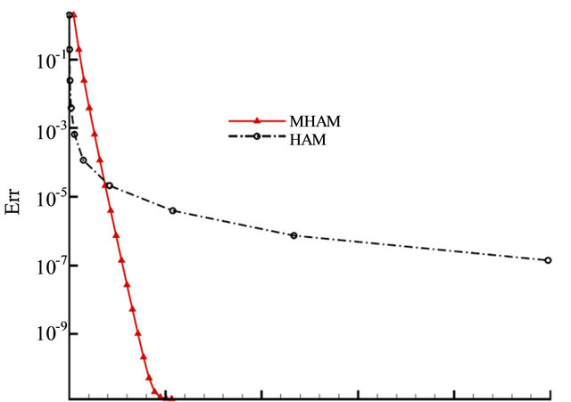
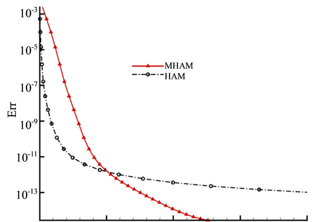
and  given by MHAM are almost the same as that given by standard HAM. From Table 3, we can see that the number of terms in high-order approximation given by MHAM is 39, while that given by HAM grows exponentially. Moreover, it shows that MHAM needs less than ninth the CPU time used by HAM to get 50th-order approximate solution. The curve of residual error and CPU time is plotted in Figure 1. From it we can see that the truncation technique greatly improves the efficiency of HAM.
3.2. Example 2
Consider a set of two coupled nonlinear differential equations (see Kuiken [10] for details)
 (18)
(18)
 (19)
(19)
with the boundary conditions
 ,
,  ,
,  where
where ![]() is the Prandtl number.
is the Prandtl number.
Under the transformation
 ,
,  Equations (18) and (19) become
 , (20)
 , (21)
with the boundary conditions
Table 1. Comparison of  given by MHAM and HAM in Example 1.

Table 2. Comparison of  given by MHAM and HAM in Example 1.

Table 3. Comparison of CPU time (seconds) and number of terms appearing in mth order approximation given by MHAM and HAM in Example 1.

0 500 1000 1500 2000 2500 CPU (s)
Figure 1. Residual error versus CPU time in Example 1. Solid line: MHAM; Dash-dotted line: HAM.
 ,
,  ,
, .
.
We seek the solution and
and in the form
 ,
,  where
where ,
,  are coefficients.
Following Liao [2], the auxiliary linear operators are chosen as

 ,
, 
and the initial guess of  and
and  as
as
 ,
, .
.
Then the high-order deformation equations become
 ,
,
 subject to the homogeneous boundary conditions
 and
and
 ,
,
 .
.
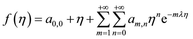
We find that  and
and  can be expressed in the form of finite combination of functions
 , (22)
and
 , (23)
respectively. Applying the Schmidt-Gram process to the first  functions in (22) and (23), respectively, we obtain two set of N orthonormal functions, denoted by
  and
and . We use
  to approximate
  every time it is got, and
  to approximate
 . Then
  and
and  are used to proceed the computation.
In the experiment, we set ,
,  ,
,  ,
,  ,
,  , and
, and . For different order approximation given by the two approaches, the quantity
  is showed in Table 4, and the residual error for Equation (20) is compared in Table 5. We can see that although we use
  to proceed the computation instead of
 , the accuracy of the approximate solution is well retained. From Table 6, we can see that the number of terms in the high-order approximation given by MHAM was kept within 16, while that
Table 4. Comparison of  given by MHAM and HAM in Example 2.

Table 5. Comparison of  given by MHAM and HAM in Example 2.
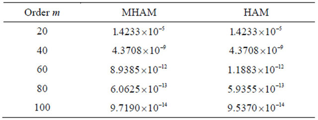
Table 6. Comparison of CPU time (seconds) and number of terms appearing in  given by MHAM and HAM in Example 2.

given by HAM grows with the order![]() . Moreover, it shows that MHAM needs less CPU time than the standard HAM to get high-order approximate solution. The curve of residual error and CPU time is plotted in Figure 2. From it we can see that the truncation technique is more powerful to get higher-order approximation than the standard HAM.
. Moreover, it shows that MHAM needs less CPU time than the standard HAM to get high-order approximate solution. The curve of residual error and CPU time is plotted in Figure 2. From it we can see that the truncation technique is more powerful to get higher-order approximation than the standard HAM.
4. Conclusion and Discussions
In this paper, an efficient modification of HAM is proposed for solving boundary layer problems. Using the derived orthonormal functions, the right-hand sides of highorder deformation equations are approximated to reduce the rapid growth of terms in high-order approximate solution. Two typical examples show that the new approach can greatly reduce the terms in the approximate solution; meanwhile the accuracy can be largely retained. The new approach needs less time to get high-order approximation than the standard HAM. However, one unsolved problem
0 50 100 150 200 CPU (s)
Figure 2. Residual error versus CPU time in Example 2. Solid line: MHAM; Dash-dotted line: HAM.
of this approach is that there is so far no estimation theory on how many orthonormal functions should be used to approximate  when accuracy is prior given. We will try to generalize this truncation technique to solve PDEs in the next step.
5. Acknowledgements
The first author would like to thank Dr. Z. Liu for valuable discussion. This work is supported by State Key Laboratory of Ocean Engineering (Approve No. GKZD- 010053).
REFERENCES
- S. Liao, “Proposed Homotopy Analysis Techniques for the Solution of Nonlinear Problem,” Ph.D. Thesis, Shanghai Jiao Tong University, Shanghai, 1992.
- S. J. Liao, “Beyond Perturbation: Introduction to the Homotopy Analysis Method,” Chapman & Hall/CRC, Boca Raton, 2003.
- K. Yabushita, M. Yamashita and K. Tsuboi, “An Analytic Solution of Projectile Motion with the Quadratic Resistance Law Using the Homotopy Analysis Method,” Journal of Physics A: Mathematical and Theoretical, Vol. 40, No. 29, 2007, pp. 8403-8416. doi:10.1088/1751-8113/40/29/015
- V. Marinca and N. Herisanu, “Application of Optimal Homotopy Asymptotic Method for Solving Nonlinear Equations Arising in Heat Transfer,” International Communications in Heat and Mass Transfer, Vol. 35, No. 6, 2008, pp. 710-715. doi:10.1016/j.icheatmasstransfer.2008.02.010
- Z. Niu and C. Wang, “A One-Step Optimal Homotopy Analysis Method for Nonlinear Differential Equations,” Communications in Nonlinear Science and Numerical Simulation, Vol. 15, No. 8, 2010, pp. 2026-2036. doi:10.1016/j.cnsns.2009.08.014
- S. Liao, “An Optimal Homotopy-Analysis Approach for Strongly Nonlinear Differential Equations,” Communications in Nonlinear Science and Numerical Simulation, Vol. 15, No. 8, 2010, pp. 2003-2016. doi:10.1016/j.cnsns.2009.09.002
- Z. Lin, “Research and Application of Scaled Boundary FEM and Fast Multipole BEM,” Ph.D. Thesis, Shanghai Jiao Tong University, Shanghai, 2010.
- S. Liao, “Notes on the Homotopy Analysis Method: Some Definitions and Theorems,” Communications in Nonlinear Science and Numerical Simulation, Vol. 14, No. 4, 2009, pp. 983-997. doi:10.1016/j.cnsns.2008.04.013
- S. J. Liao, “A Uniformly Valid Analytic Solution of TwoDimensional Viscous Flow over a Semi-Infinite Flat Plate,” Journal of Fluid Mechanics, Vol. 385, 1999, pp. 101-128. doi:10.1017/S0022112099004292
- H. K. Kuiken, “A Backward Free-Convective Boundary Layer,” The Quarterly Journal of Mechanics and Applied Mathematics, Vol. 34, No. 3, 1981, pp. 397-413. doi:10.1093/qjmam/34.3.397