Open Journal of Modern Hydrology
Vol.3 No.4(2013), Article ID:37539,9 pages DOI:10.4236/ojmh.2013.34022
A Structural Overview through GR(s) Models Characteristics for Better Yearly Runoff Simulation
![]()
1National Researches Institute of Water, Forests and Rural Engineering, Tunis, Tunisia; 2National Water Distribution Utility, Tunis, Tunisia; 3Food and Agriculture Organisation, Addis-Abeba, Ethiopia.
Email: mouelhi@gamail.com
Copyright © 2013 Safouane Mouelhi et al. This is an open access article distributed under the Creative Commons Attribution License, which permits unrestricted use, distribution, and reproduction in any medium, provided the original work is properly cited.
Received June 13th, 2013; revised July 13th, 2013; accepted July 20th, 2013
Keywords: Time Step; Runoff-Rainfall; GR(s) Models; Yearly; Monthly; Daily
ABSTRACT
In rainfall-runoff modelling, a monthly timescale and an annual one are sufficient for the management of deductions. However, to simulate the flow at a large time-step (annual), we generally precede the use of a model working for a finer time-step (daily) while aggregating the desired outputs. The finest time-steps are considered, apriori, as the most performant. By passing from one time-step to another, and in order to work in the desired time-step (annual) and calculate the potential gains or loss, this article proposed a comparative study between the aggregation method of outputs of a modal working at a finer time step, and a method in which we use a conceived model from the beginning. To ensure this comparative and empirical approach, the choice has been focused on (GRs) models to a daily time-step (GR4J), monthly time step (GR2M) and annual time step (GR1A). The modelling platform used is the same for all three models taking into account the specificities of each one: the same data sample, the same optimization method, and the same function criterion are used during the construction of these models. Due to the moving between these time steps, results show that the best way to simulate the annual flow is to use an appropriate and designed modal initially conceived to this time step. Indeed, this simulation seems to be less effective when using a model at a finer time-step (daily).
1. Introduction
The hydrological literature is rich in conceptual rainfallrunoff models at different time steps especially the daily one such as Beven and Kirkby [1], Thomas [2], Milly [3], Vandewiele et Xu, 1994 [4], Bergström [5], Perrin et al. [6], Mathevet [7], Mouelhi et al. [8,9].
The approach consists in passing from a large timestep to a finer one or vice versa, in order to calibrate the parameters, optimize the functions of the modals, or test the interdependence of parameters of the same model from one time-step to another, which is increasingly adopted: Hughes [10], Nalbantis [11], Kavetski et al. [12], Haddeland et al. [13], Littlewood and Croke [14], Kling and Nachtnebel [15], Widen-Nilsson et al. [16], Clark and Kavetski [17].
However, to simulate the flows at a larger time-step (monthly or annually), we often use a rainfall-runoff model operating at a daily time-step, then, by the aggregation of outputs, we obtain the flows at the desired one (monthly, seasonal, annual).
This method results from “the received” idea of the structural superiority of modals performing at finer timestep (daily or hourly) compared to others at a larger one.
However, this summing method of models’ output has not been compared to the method where appropriate modals at a desired time-step are applied. Is it always effective? Which model can we choose? And for which timestep? Passing from one time-step to another, what is the evolution of the structural morphology of the modelling conceptual globing rainfall-runoff?
While trying to encrypt the gain or loss, this article attempts to answer these questions. It is caused by the use of a model to estimate the flow rates on a time-step higher than that for which the modal is conceived to work.
This work deals with the case of the annual time step, where the flows are simulated: either by an annual model; or monthly or daily models when aggregating the outputs to the annual time step.
The first paragraph deals with the choice of the model, which is brought to GRs models (GR4J, GR2M and G1A). The second one is devoted to explain the platform of the used modelling for the three time-steps. In this section, a new method of initialization has been tested. The last paragraph explains and interprets results.
2. The Chosen Models: GR(s)
The choice of GR(s) models compared to others is based on the following reasons: the availability of a model at each time-step. Same modelling platform, (sample data and modelling methodology) used in their construction, and better performance compared to other global conceptual models.
2.1. Daily Time-Step GR4J (Perrin et al., 2003)
GR4J is a global conceptual rainfall-runoff model with four free parameters. It is the result of gradual improvements of the work undertaken within the National Research Institute of Science and Technology for Environment and Agriculture “IRSTEA”: Michel [18], Edijatno and Michel [19], Edijatno [20], Edijatno et al. [21], Rakem [22], Perrin [23], Perrin et al. [24].
The version used in this article is the one proposed by Perrin. It is deducted following a comparative and empirical approach among 38 global conceptual models including TopModel, HBV, etc. [24].
The structure of GR4J model is based on a reservoir of production called also “Reservoir-Soil”, a reservoir of draining, and on two Unitarian hydrographs (Figure 1).
Pluviometry (P) and potential evapotranspiration (E), expressed in millimetres (mm), are inputs’s variables of the model. The interception phase consists in calculating,

Figure 1. Architecture of GR4J model.
from these two inputs, the net rain (Pn) or the net evapotranspiration (En) as follows (Equation (1)):
 (1)
(1)
The Soil Reservoir is characterized by its maximum capacity “X1”, the first parameter of GR4J model. (S) is the reservoir content responsible for realizing a follow-up of humidity in the basin.
In the case where all the rain is consumed during the interception, the amount (En) is used to evaporate the water in the reservoir-ground at a real rate (Es). Conversely, when rain remains (Pn), a part of it (Ps) is stored in the reservoir. (Es) and (Ps) are calculated as functions of filling rate of the reservoir of production
 (1)
(1)
The content of the reservoir of production is updated as follows
 (3)
(3)
A percolation term, which is the reservoir output and the function of the S' level, feeds the flow as follows (Equation (4)):
 (4)
(4)
The content of the reservoir is updated again (Equation (5))
 (5)
(5)
The supplementary part of rain (Pn – Ps) or effective rainfall, to which we add the percolation term, is separated into two components. A direct flow (Q1), which represents 10% of the effective rainfall, joins the outfall after a rooting by a Unitarian hydrograph (SH2). The other part (Q9) representing 90% of the effective rainfall is routed by another Unitarian hydrograph (SH1) followed by a rooting reservoir.
The Unitarian hydrograph is a function that allows the creation of a time lag between rainfalls and flows. The two used hydrographs (SH1 and SH2) depend on the same reference period. (X3), as a third parameter wedged from the model, characterizes the rising time of the Unitarian hydrograph. Expressions of functions (SH1) and (SH2) are as follows (Equation (6)):
 (2)
(2)
(j) can also take non-integer values. Hydographs’s ordinates (UH1 and UH2) are calculated from curves in “S” representing the cumulation of Unitarian rainfall proportion by the hydrograph in function of time, noting respectively SH1 and SH2 (Equation (7)):
 (3)
(3)
At each time step (i), outputs (Q9) and (Q1) of the two hydrographs are calculated by (Equation (8)):
 (8)
(8)
The (Q9) quantity passes through a non-linear rooting reservoir of level (R) and of maximum capacity (X2) which is the second parameter to wedge from the model. This reservoir is characterized by its act of instant draining of this type: “Qr(t) = K∙(R(t))5”, wherein (K) is a constant. The level (R) of the rooting reservoir is affected by the relative quantity in underground exchanges, which is a function of the fourth parameter of the model (X4).
 (9)
(9)
The level (R) of draining reservoir is updated as in the Equation (10)
 (10)
(10)
Having transited the rooting reservoir, the quantity is deducted by the integration of the draining act as follows (Equation (11))
 (11)
(11)
The level of the reservoir is updated according to the Equation (12)
 (12)
(12)
Having undergone the hydrograph action (HU2), the quantity (Q1) is subject to the same changes to give the flow component according to Equation (13):
 (13)
(13)
The flow is then given by the Equation (14):
 (14)
(14)
2.2. Monthly Time-Step: GR2M (Mouelhi et al., 2006b)
The (G2M) is a global conceptual model with two parameters. As for the GR4J case, it has underwent many transformations since its first construction up to the most recent version Edijatno [25], Kabouya [26], Kabouya and Michel [27], Makhlouf [28], Makhlouf and Michel [29], Nascimento [30], Mouelhi [31], Mouelhi et al. [8].
The most recent structure has been developed using a “step by step” approach or “stepwise approach”. It is a question of testing a multitude of interconnected components and retaining only the combination leading to a better performance [8].
Empirically, and further to a comparative study with eight other structures of global conceptual rainfall-runoff models, the GR2M model seems to be the most performant.
This model is characterized by two functions (Figure 2): 1) a function of production that revolves around a reservoir-ground of a maximum capacity (X1), which is the first parameter to be wedged. Transferring a percolation of reservoir-ground is ensured by a dependent feature of the stock status “S”; 2) a transfer function represented by a quadratic draining reservoir of a capacity fixed to 60 mm.
This reservoir is modified by an underground exchange, whose coefficient (X2) is the second parameter to optimize. The runoff is calculated according to seven operations (Equations (15)-(24)): Under the action of rainfall (P), Sm−1 level becomes S*, where (m) refers to the month in question:
 (15)
(15)
It follows a contribution to the (PR) flow:

Figure 2. Architecture of GR2M model (Mouelhi, 2003; Mouelhi et al., 2006b).
 (16)
(16)
(1) Under the action of potential evapotranspiration (ET), the level (S*) becomes (S**) as follows:
 (17)
(17)
(2) By percolation (S**) becomes (Sm) at the end of the month (m):
 (18)
(18)
 (19)
(19)
(3) The reservoir (R), which level at the beginning of the month (Rm−1) becomes (R*):
 (20)
(20)
(4) The exchange term (ECH) is calculated as follows, where (X2) is a positive and dimensionless parameter:
 (21)
(21)
(5) Under the action of this exchange, the reservoir level becomes:
 (22)
(22)
(6) The rooting reservoir has a fixed capacity equal to 60 mm. It drains according to a quadratic law
 (23)
(23)
(7) After draining the level of the reservoir, the m month becomes:
 (24)
(24)
2.3. Annual Time-Step: GR1A (Mouelhi et al., 2006a)
The GR1A model was built by testing numerous junctions of components stemming from finer and bigger time-step: multiannual, monthly and daily, [9] and [31]. The form is found with a single parameter. It seems very simple where hydrological concepts no longer appear (Equation (25)):
 (25)
(25)
Qk: the simulated flow of the year k. Pk: the observed rainfall of the year k. Pk−1: the amount of the observed rainfall of the year k−1. Ek: the amount of potential evapotranspiration of the year k. The parameter of the model to be optimized.
3. Modelling Platform
To insure the passage from one time-step to another without biasing results, the modelling platform used during the construction of these modals is the same used in this work.
3.1. Sample Data
The sample data used in this study is 407 watersheds having served in modelling work conducted at (IRSTEA), including the development of models GR4J, GR2M and GR1A: Mouelhi et al. [8] and [9], Perrin [23], Perrin et al. [24], Makhlouf and Michel [27], Makhlouf [28], Mouelhi [31], Andréassian [32], Andréassian et al. [33]; Perrin et al. [34].
This sample collects rainfall data (P), of an evapotranspiration (E) and flow (Q) of very varied hydroclimatic conditions of 407 watersheds of: 298 French basins, 70 Americans, 26 Australians, 9 Ivorian and 4 Brazilian. (Table 1).
The rainfall data (P), of flow (Q) and some of the potential evapotranspiration data (E) are provided to a daily time-step. It was necessary to aggregate data at different

Table 1. Sample statistics characteristics of data.
desired time-steps to meet the objectives of this work.
This sample presents quite different climatological, hydrological and anthropogenic conditions. On one hand, there exist semi-arid conditions in Australia or in the south of the United States, with watercourses knowing flows only a few days in the year. On the other hand, we find wet tropical conditions in the south of the Ivory Coast or the North of Australia.
The French basins are characterized by a quiet big climatic diversity, with Mediterranean and continental influences.
The watershed size varies over a wide range, from 0.1 to more than 50,000 km2. The larger watersheds are those of La Seine in Paris (43,800 km2) and of São Francisco in the dam of Três Marias in Brazil (50,600 km2).
This sample also reflects a variety of seasonal patterns. Indeed, basins exist with very contrasted wet and dry seasons and also fairly unfirming scheme throughout the year both at the level of rainfall and flow.
3.2. Methodology of the Application of Models
3.2.1. Variable Target, Assessment Criteria and Optimization Method
The objective behind choosing the variable target is to take into account, in a balanced way, the different ranges of elapsed flows without favouring the quality of reproduction of low or strong values.
However, residues of a model are generally not homoscedastic that is to say, their variance is dependent on the value of the flow [32].
If the choice of variable target has been on the flows (Q), strong yield basins would have been privileged. The interest is proceeding by a transformation on variable flow (Q) in order to take into account, in a relatively uniforming way, all the orders of High flows.
The flow rate could be an appropriate choice of transformation. This variable tends to take into account the humid and arid basins in an equivalent manner. Yet, during the measures, the flow, as well as the pluviometry, are tainted by error. Dividing the flow by rainfall, the relative errors accumulate. Thus, the risk of biased estimates is even stronger.
A logarithmic transformation on flows, to which we add a low constant to avoid the problem of the useless flows, could be valid [35].
So, values of flows will be levelled, and errors of the model vary then in the same height order for all classes of flows.
A transformation power of flows (transformation with 0.5 power), allows to have the intermediate case between the logarithmic transformation and the solution (Q) without biasing calculations [36].
Such a choice of transformation allows, at the same time, to reduce the character of non-homoscedasticity residue models, and to keep the works having served in the construction of coherent used models in this article. Consequently, it is the variable “root of Q” that is used.
The criterion function used is based on the so-called Nash Criterion (CN) [37]. When performing the chosen transformation (Q root), for each watershed. This criterion can be written as follows (Equation (26)):
 (26)
(26)
N: total number of calculated and observed values for each watershed. Q: observed and calculated runoff depth (in millimetres per time-step). : runoff depth estimated by this model (in millimetres per time-step).
 : average over N of the square root values of the observed water passed runoff depth.
(CN) will take values from (−∞ to 1). The model is considered as performant when the estimated flows get closer to the observed flows, that is, when CN is close to 1.
Previous studies have demonstrated the relevance of this criterion relative to another part of the overall conceptual modelling [38].
The choice of the optimization method has been focused on the so-called “step by step” (Michel et al., 1989; Nascimento, 1995). It is a direct method, which operates a local optimization (maximization or minimization) of an objective function chosen by the user regardless of the method.
This is a maximization of the (CN) function. This method adopts a displacement strategy along the axes of the parameter space, with a research step that can vary from one iteration to another. It proved a better performance compared to other methods in the context of global conceptual rainfall-runoff modelling [23].
3.2.2. Implementation and Evaluation of the Robustness
The robustness models was assessed using the technique of the “double sample”, also called “Split-Sample test” [39]. It is a question of cutting the period of observation into two sub-periods, one for the wedging and the other one for the control (or validation). Their roles will be swapped so that we have two periods of stalling and two periods of controls. Thus the model tested will be evaluated only at the control.
For each watershed, “Nash” corresponds to the sum of the squared deviations between observed and calculated values relative to the first and the second control, with regard to the sum of squares of distances between the value and average observed over all the period of observation (wedging and control). It is translated according to the following formulation (Equation (27)):
 (27)
(27)
CNSS: Nash criterion using the “Split-Sample” technique. N1: start-up time. N2: end of the first sub-period. N: total observation period (day for GR4J, Months for GR2M and year for GR1A for each watershed:  average of
  observed in all period’s totality. Q: the observed runoff depth.
 : Calculated water blade by the modal. And {S}0: the initial state of the system.
The initial state of the system consists in predefining values of departure for the parameters of the model before passing to the optimization phase. In other, words before its confrontation to the observed hydrological reality.
In the case where the model would contain reservoirs, this initialization phase would also consist in predefining the initial levels of these before the wedging.
In an empirical or conceptual modelling, this initialization phase appears as a “physical”: necessity: “It is better to know from where we start to understand where we are going.”
Generally, this initial state is defined arbitrarily by the modeller. However, the initial state choice can influence the optimal set of parameters of the model and its performance. To overcome this constraint, we usually choose a period of initiation, which consists in turning the system for an observation period without being taken into account in the calculation of the performance.
For better daily time-step, the starting period, associated with the best performance, is of one year, that is to say, 365 observations (Perrin, 2000; Perrin et al., 2001). It is the same period used in this article for the same time-step.
At the monthly time step, a year of commissioning is equivalent to only 12 observations. To mulch this problem, a new method has been tested, here by the “starting up of cyclic system”.
This latter consists in feeding the reservoir(s) by an interannual monthly rainfall. The equivalent output is the average of interannual monthly flows (Figure 3). The operation is repeated until the stabilization of the reservoir level. The corresponding level will be taken as the initial level of it.
The calculations showed that 20 iterations of cyclic regime with one effective year of starts are sufficient at a monthly time-step. As for the annual one, the modal chosen here is without reservoir (Equation (25)). It will be enough to fix the initial value of the parameter by avoiding the mathematically insensible zones (not near zero and infinity).
4. Results and Discussion
Given large number of tests in wedging and controlling as for a used model, 814 wedgings, 814 controls and 407 values of criterion of performance, it was interesting to be able to analyse the results of the performance of each model, by summarizing it into one or two numbers.
The quantile (30%) of performances distribution has been mainly chosen, noted (Cr3) as well as the average of the values of CNSS. These distributions are obtained by ranking CNSS criterion values of a model in control through ascending and constructing the corresponding experimental distribution.
First of all, the GR1A model was applied on the sample data to encrypt its performance. Then, with monthly data on the same sample, GR2M monthly model was used, where annual rates were estimated by summing the outputs. Similarly, annual rates were also estimated from daily data by using GR4J model (Figure 4 and Table 2).
As reported, and strongly influenced by negative values of the performance criterion, the 30% quantile (CR3) is adopted here as a criterion in addition to the average (Table 2). These criteria are also argued in Figure 4 in order to get an overall idea of the performance of models over the entire sample data.
The annual model GR1A widely outclasses the daily model GR4J, and less clearly the model GR2M. These results show that, to feign annual flows, the best way is to use a model suited to this time-step, by avoiding getting lost in useless details that can weight down the task

Figure 3. Cyclic started regime.
of regrouping data and the implementation of the model.
This report comes against the preconceived ideas to use a finer model and to aggregate the data of outputs for every desired time-step.
However, from the at about 60% quantile, (CR6), the performance of annual, monthly and daily models become comparable with a slight superiority of GR4J then GR2M compared to GR1A (Figure 4). This could be explained by the fact that the distribution of rainfall and evapotranspiration over the year is not reflected in the architecture of GR2M and GR1A models.
Indeed, for arid or semi-arid watersheds, rainy season is concentrated in few months or even few days of the year.
On the other hand, to visualise the morphology of models from one time to another, the GR4J, GR2M and GR1A architectures have been gathered on the same figure (Figure 5). The daily and monthly models are relatively connected to the conceptual plan.
This conceptualization disappears completely at an annual time-step. Only the underground exchange, taking the form of a linked coefficient to the evapotranspiration cinquefoil, remains. Thus, the passage from monthly time-step to yearly time step is done “brutally”.

Table 2. Performances of the GR4J and GR2M models at the yearly time step.
We believe that the prospect of building a global conceptual model at a seasonal time-step seems to be interesting. Conceptually, it will allow to see the composition of a model opening at an intermediate time step between the monthly and the annual.
Furthermore, the contrast between dry and wet seasons will be taken into account, which is not considered at the level of GR2M and GR1A architectures.
5. Conclusions
A modelling methodology was adopted to avoid biasing results and to encrypt the gain or loss caused by the use of a model, in order to estimate the flow at a time-step higher than that to which the modal is conceived to operate.
So, the choice of models is carried to GR1A, GR2M and GR4J, where the modelling platform is opted here. It also has been used to their constructions: sample data (407 watersheds), performance criterion of Nash by introducing a technique called “Split-Sample” (CNSS), variable target (root flows) and optimization method (step by step).
Let us note here that a new initialization technique of reservoirs’ levels, called “cyclic start-up scheme” allowed the escape at their arbitrary choices.
Contrary to preconceived ideas, results show that the use of a designed model working at a large time-step (GR1A for the annual), is more accommodated than the use of a finer model (GR2M or GR4J) by aggregating the exits at an annual time-step.
Structurally, the conceptualization of models disappears at an annual time-step (GR1A) compared to daily and monthly time-steps (GR2M and GR4J), which remain relatively similar structures.

Figure 4. Comparison of G4J, GR2M and GR1A model performance at the annual time step.
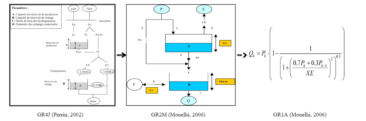
Figure 5. The GR(s) models architecture overview.
It seems to be interesting then to build a model at a seasonal time-step (intermediate between the monthly and the annual), which will take into account the effect of rainfall distribution and evapotranspiration throughout the year.
REFERENCES
- K. J. Beven and M. J. Kirkby, “A Physically Based, Variable Contributing Area Model of Basin Hydrology,” Hydrological Sciences Bulletin, Vol. 24, No. 1, 1979, pp. 43-69. http://dx.doi.org/10.1080/02626667909491834
- H. A. Thomas, “Improved Methods for Rational Water Assessment,” Water Resources Council, Washington DC, 1981.
- P. C. D. Milly, “Climate, Interseasonal Storage of Soil Water, and the Annual Water Balance,” Water Resources Research, Vol. 17, No. 1-2, 1994, pp. 19-24. http://dx.doi.org/10.1029/94WR00586
- C. Y. Xu and G. L. Vandewiele, “Parsimonious Monthly Rainfall-Runoff Models for Humid Basins with Different Input Requirements,” Advances in Water Resources, Vol. 18, No. 1, 1995, pp. 39-48.
- S. Bergström, “The HBV Model,” In: V. P. Singh, Ed., Computer Models in Watershed Modeling, Water Resources Publications, Highlands Ranch, Colorado, 1995, pp. 443-476.
- C. Perrin, C. Michel and V. Andréassian, “Improvement of a Parsimonious Model for Streamflow Simulation,” Journal of Hydrology, Vol. 279, No. 1, 2003, pp. 275-289. http://dx.doi.org/10.1016/S0022-1694(03)00225-7
- T. Mathevet, “Which Global Rainfall-Runoff Models in an Hourly Time Step? Development and Empirical Comparison of Models on a Large Sample of Watersheds,” Ph.D. Thesis, AgrosParisTech (Ex. ENGREF), 2005, 463 p.
- S. Mouelhi, C. Michel, C. Perrin and V. Andréassian, “Stepwise Development of a Two-Parameter Monthly Water Balance Model,” Journal of Hydrology, Vol. 318, No. 1-4, 2006, pp. 200-214. http://dx.doi.org/10.1016/j.jhydrol.2005.06.014
- S. Mouelhi, C. Michel, C. Perrin and V. Andréassian, “Linking Stream Flow to Rainfall at the Annual Time Step: The Manabe Bucket Model Revisited,” Journal of Hydrology, Vol. 328, No. 1-2, 2006, pp. 283-296. http://dx.doi.org/10.1016/j.jhydrol.2005.12.022
- D. A. Hughes, “Variable Time Intervals in Deterministic Hydrological Models,” Journal of Hydrology, Vol. 143, No. 3-4, 1993, pp. 217-232. http://dx.doi.org/10.1016/0022-1694(93)90193-D
- I. Nalbantis, “Use of Multiple-Time-Step Information in Rainfall-Runoff Modeling,” Journal of Hydrology, Vol. 165, No. 1, 1995, pp. 135-159. http://dx.doi.org/10.1016/0022-1694(94)02567-U
- D. Kavetski, G. Kuczera and S. W. Franks, “Semidistributed Hydrological Modeling: A ‘Saturation Path’ Perspective on TOPMODEL and VIC,” Water Resources Research, Vol. 39, No. 9, 2003, p. 1246. http://dx.doi.org/10.1029/2003WR002122
- I. Haddleland, D. P. Lettenmaier and T. Skaugen, “Reconciling Simulated Moisture Fluxes Resulting from Alternate Hydrologic Model Time Steps and Energy Budget Closure Assumptions,” American Meteorological Society, Vol. 7, No. 3, 2006, pp. 355-370.
- I. G. Littlewood and B. F. W. Croke, “Data Time-Step Dependency of Conceptual Rainfall—Stream Flow Model Parameters: An Empirical Study with Implications for Regionalization,” Hydrological Sciences Journal, Vol. 53, No. 4, 2008, pp. 685-695. http://dx.doi.org/10.1623/hysj.53.4.685
- H. Kling and H. P. Nachtnebel, “A Spatiotemporal Comparison of Water Balance Modeling in an Alpine Catchment,” Hydrological Processes, Vol. 23, No. 7, 2009, pp. 997-1009. http://dx.doi.org/10.1002/hyp.7207
- E. Widen-Nilsson, L. Gong, S. Halldin and C.-Y. Xu, “Model Performance and Parameter Behavior for Varying Time Aggregations and Evaluation Criteria in the WASMOD-M Global Water Balance Model,” Water Resources Research, Vol. 45, No. 5, 2009, 14 p. http://dx.doi.org/10.1029/2007WR006695
- M. P. Clark and D. Kavetski, “Ancient Numerical Daemons of Conceptual Hydrological Modeling: 1. Fidelity and Efficiency of Time Stepping Schemes,” Water Resources Research, Vol. 46, No. 10, 2010, 23 p. http://dx.doi.org/10.1029/2009WR008894
- C. Michel, “What Can We Do in Hydrology with a Conceptual Model with One Parameter?” La Houille Blanche, No. 1, 1983, pp. 39-44.
- Edijatno and C. Michel, “A Rainfall Runoff Model with Three Parameters,” La Houille Blanche, No. 2, 1989, pp. 113-121.
- Edijatno, “Development of a Basic Rainfall-Runoff Model to Daily Time,” Ph.D. Thesis, Louis Pasteur University/ENGEES, Strasbourg, 1991.
- Edijatno, N. O. Nascimento, X. Yang, Z. Makhlouf and C. Michel, “A Daily Watershes Model with Three Free Parameters,” Hydrological Sciences Journal, Vol. 44, No. 2, 1999, pp. 263-277. http://dx.doi.org/10.1080/02626669909492221
- Y. Rakem, “Critical Analysis and Mathematical Reformulation of Empirical Rainfall-Runoff (GR4J) Model,” Ph.D. Thesis, Ecole Nationale des Ponts et Chaussées, Paris, 1999.
- C. Perrin, “To an Improvement of a Lumped RainfallRunoff Model through a Comparative Approach,” Ph.D. Thesis, Institut National Polytechnique de Gronoble, Gronoble, 2000.
- C. Perrin, C. Michel and V. Andréassian, “Improvement of a Parsimonious Model for Streamflow Simulation,” Journal of Hydrology, Vol. 279, No. 1, 2003, pp. 275-289. http://dx.doi.org/10.1016/S0022-1694(03)00225-7
- Edijatno, “Improvement of a Simple Rainfall Runoff Model at a Daily Time Step on Small Watersheds,” Master Report, Cemagref Publication, 1987, 45 p.
- M. Kabouya, “Rainfall—Runoff Modeling at Monthly and Annual Time Step in Northern Algeria,” Ph.D. Thesis, Université Paris Sud, Laboratoire d’Hydrologie et de Géochimie Isotopique d’ORSAY, Paris, 1990, 374 p.
- M. Kabouya and C. Michel, “Estimation of Surface Water Resources at Monthly and Annual Time Step, Application to a Semi-Arid Country,” Revue des Sciences de l’Eau, Vol. 4, No. 4, 1991, pp. 569-587. http://dx.doi.org/10.7202/705116ar
- Z. Makhlouf, “Supplements on the GR4J Rainfall-Runoff Model and Estimation of Its Parameters,” Ph.D. Thesis, Paris XI Orsay, Cemagref, 1993.
- Z. Makhlouf and C. Michel, “A Two-Parameter Monthly Water Balance Model for Frensh Watersheds,” Journal of Hydrology, Vol. 162, No. 3-4, 1994, pp. 199-318. http://dx.doi.org/10.1016/0022-1694(94)90233-X
- N. O. Nascimento, “Assessment Using an Empirical Model of Human Actions Affect on the Rainfall-Runoff Relationship in Watershed Scale,” Ph.D. Thesis, ENPC, Paris, 1995.
- S. Mouelhi, “Towards a Coherent Chain of Global Conceptual Rainfall-Runoff Models at Multiyear, Yearly, Monthly and Daily Time Steps,” Ph.D. Thesis, Ecole Nationale du Génie Rural, des Eaux et Forêts, Paris, 2003.
- V. Andréassian, “Impacts of Forest Cover Change on the Hydrological Behavior of Watersheds,” Ph.D. Thesis, Université de Pierre et Marie Curie Paris VI, Paris, 2002.
- V. Andréassian, C. Perrin, C. Michel, I. Usart-Sanchez and J. Lavabre, “Impact of Imperfect Rainfall Knowledge on the Efficiency and the Parameters of Watershed Models,” Journal of Hydrology, Vol. 250, No. 1, 2001, pp. 206-223. http://dx.doi.org/10.1016/S0022-1694(01)00437-1
- C. Perrin, L. oudin, V. Andreassian, C. Rojas-Serna, C. Michel and T. Mathevet, “Impact of Limited Streamflow Data on the Efficiency and the Parameters of Rainfall—Runoff Models,” Hydrological Sciences Journal, Vol. 52, No. 1, 2007, pp. 131-151. http://dx.doi.org/10.1623/hysj.52.1.131
- B. Ambroise, J. L. Perrin and D. Reutenauer, “Multicriterian Validation of a Semi-Distributed Conceptual Model of the Water Cycle in the Fecht Catchment (Vosges Massif, France),” Water Resources Research, Vol. 31, No. 6, 1995, pp. 1467-1481. http://dx.doi.org/10.1029/94WR03293
- F. H. S. Chiew, M. J. Stewardson and T. A. McMahon, “Comparison of Six Rainfall-Runoff Modeling Approaches,” Journal of Hydrology, Vol. 147, No. 1-4, 1993, pp. 1-36. http://dx.doi.org/10.1016/0022-1694(93)90073-I
- J. E. Nash and J. V. Sutcliffe, “River Flow Forecasting Through Conceptual Models. Part I—A Discussion of Priciples,” Journal of Hydrology, Vol. 27, No. 3, 1970, pp. 282-290. http://dx.doi.org/10.1016/0022-1694(70)90255-6
- E. Servat, A. Dezetter and J. M. Lapetite, “Study and Selection of Calibration Criteria of Rainfall-Runoff Models,” IRD (ex. ORSTOM), Note 2, Programme ERREAU, IRD Publication, Montpellier, 1989.
- V. Klemes, “Operational Testing of Hydrological Simulation Models,” Journal of Hydrological Sciences, Vol. 31, No. 1, 1986, pp. 13-24. http://dx.doi.org/10.1080/02626668609491024