Received 8 February 2016; accepted 17 March 2016; published 22 March 2016

ABSTRACT

This report describes a fundamental model of a quantum circuit for finding complex eigenvalues of Hamiltonian matrices on the quantum computers through the use of an iteration algorithm for estimation of the phase. In addition to this, we demonstrate the use of the model for simulating the resonant states for quantum systems.

Keywords:

Quantum Operators, Phase Space, Quantum Circuit

1. Introduction

In the circuit model of quantum computations the change of the quantum states is implemented through quantum operators. A given algorithm, or computation, can be run on a quantum computer by using a sequence of quantum operators. These operators can be represented by unitary matrices in computational basis. These matrices represent a transformation of the linear space, the rotation is an example of such transformation. As a consequence of the transformation most of the vectors in the space are converted into new vectors, which are with a different direction. But for each transformation, there are some special vectors, which, after being transformed, continue to point in the same direction, although their length can be changed. These vectors are called eigenvectors, and the factors which depend on the change of their lengths are called eigenvalues. And now let’s look what this means in the mathematical language.

In order to transform a given vector, it must be multiplied by the transformation matrix. So, if we have a matrix H and vector ψ, the transformation vector will be Hψ. If the transformation vector has the same direction as the original vector, this is an eigenvector. Mathematically, this means that the eigenvector must be divisible to the original vector so that they can be written as Eψ, where E is a number. Thus the eigenvectors must satisfy the condition: Hψ = Eψ.

The quantum state is something that encapsulates the entire necessary information for the physical system. Moreover, the quantum system has an infinite number of possible states, but they all can be expressed as linear combinations from a certain number of base states. For example, if the states are marked with kets (|∙∙∙⟩), then they can be used numbered kets (, , etc.) in order to be designated the base states, after which the total ket may be expressed as: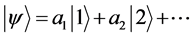. The base states could be designated as single directions:, , and the expression for the general state would have been:.

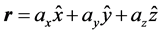Regardless of the type of the states, the coefficient a_i can be stored in a vector,

or

If the vector is an eigenvector of any matrix, then the state, which corresponds to the vector, is an eigenstate of the operator, which corresponds to the matrix.

Although this unitary image is suitable for many tasks, it prevents the application of a quantum computation at new tasks, where the computations can only be described through Hamiltonian matrices. In addition, each attempt for approximation of those Hamiltonian parts will affect negatively on the accuracy of the results. The model of the circuit, created for the Harrow et al.’s algorithm [1] [2] , uses an approximation operator for the Hamiltonian parts.

It is known that the quantum algorithms are more efficient than their classic matches [3] - [5] . In certain cases, they provide exponential increase of the efficiency for simulation of the quantum systems [6] [7] . Right from the beginning the idea to make the computer compatible with the principles of the quantum theory for the simulations of the quantum systems is discussed in 1969 from Finkelstein [8] . The idea for building a computation device with a general purpose, which functions at quantum-mechanical level, is proposed for the first time from the physicist Richard Feynman in the beginning of the 80s of the 20th century [9] . At this time, there was an underlying hope that such a device may overcome the limitations of the classical computers, especially in the field of simulation of quantum-mechanical systems. Feynman [10] explained why it was impossible to be simulated a quantum system through the use of a classical computer for probability calculations. It defines a universal quantum computer that can simulate the laws of the quantum mechanics. Subsequently different models of schematic quantum algorithms have been published for the simulation of various quantum systems. Undoubtedly, the most important one of these algorithms is the algorithm for estimation of the phase [11] [12] , used for finding the eigen-energies of the relevant quantum system. The algorithm has been demonstrated experimentally for the simulation of a hydrogen molecule through the use of photonic [13] - [15] and NMR quantum computers [16] [17] . One of the postulates of the quantum mechanics states that the measurable quantities such as the energy of the stable atoms and molecules must be a Hermitian operator.

The simulation of the non-Hermitian matrices in the quantum theory requires the simulation of the Hamiltonian evolutionary matrices. However, the standard quantum computations are made by the use of unitary operators of the evolution. It has been proven that the quantum circuit can be built from Hamiltonian operators, representing quantum measurement. In addition, it was demonstrated that a specific type of single-qubit Hamiltonian operators, the controlled-NOT operators and all single-qubit unitary operators constituted a formalized group of operators for Hamiltonian quantum circuits without the need of additional qubits [18] . Some recent studies [19] proposed a quantum algorithm on the basis of measurement for finding the eigenvalues of Hamiltonian matrices. Their method uses the ideas of the conventional algorithm for estimation of the phase, the repetitive measurement, and the techniques of tomography of single-qubit states. They describe a binominal system, composed of two subsystems, in which the entire Hamiltonian includes all interacting subsystems, which indicate that different Hamiltonian matrices of the evolution can be constructed by the implementation of sequential (consecutive) projective measurements on one of these subsystems. In addition, they show that the eigenvalue of this matrix can be found in the algorithm for estimation of the phase in two different ways: through the use of tomography of the state of the qubit or with the projective measurements for a separate computation of real and imaginary parts of the eigenvalues of the Hamiltonian. However, the described in their report measurement cannot be applied deterministically. This is also a holdback for the direct application of their method to the matrix, without knowing the application of the subsystems forming the respective Hamiltonian matrix. In addition, the process of subsequent projective measurements changes the state to a large extent [20] , which affects the accuracy of the constructed non-unitary matrix, and this also reflects on the calculated eigenvalues in this method. The likelihood of success of the algorithm depends on the probability of success of the subsequent projective measurements that can decrease exponentially. The subsequent projective measurements for estimation of the phase are causing another problem―the method becomes dependent on the way of the implementation of the projective measurements.

In this report, we present a systematic approach for estimation of the complex eigenvalues of the general matrix, using а standard iteration algorithm with a programmable model of the circuit [20] - [22] . The phase values of the sought eigenvalue should be determined from the outcome of the measurement. Then, the statistical data of the measured results on the phase qubit are used for determination of the absolute value of the eigenvalue. Therefore, by the phase and the absolute value we find the complex eigenvalue of the Hamiltonian matrix. Because of the precision model of the circuit used for simulation, the proposed method gives very good results. The likelihood of success is directly dependent by the amount of ancilla qubits and decreases exponentially in size, in the cases of dense matrices. Proposed algorithm can be used as an equivalent of the main circuit for each matrix. Since the proposed model for a circuit is universal, it can be used for estimation of the eigenvalues.

In the following sections the computational model will be discussed and described in [21] - [23] . Then we explain how to use the circuit in an iteration algorithm for estimation of the phase. We discuss the algorithmic complexity and the issues about the application and compare our method with other works [19] . We will also show the application of the algorithm to the simulations of non-Hermitian quantum systems.

2. Algorithm for Computing the Eigenvalues and Vectors of a Complex Hamiltonian Matrix

We will develop a similar fast method for the finding of all eigenvalues of a complex Hamiltonian matrix M. The difference between the proposed in this publication algorithm and the known analogous ones [18] consists in the fact that here the proposed method independently generates circuit equivalents for the rows of U in separate N × N blocks with quantum operations which are then combined using a variety of states of ancilla control qubits. The method relies on unitary similarity transformations, preserving the structure of the matrix and having the desired numerical properties. The accuracy of the computed eigenvalue depends on its size, as the larger values are usually more accurate.

Let

,

where

i.e. F is the set of all complex 2n × 2n Hamiltonian matrices.

We define the set

which in fact is a set of all Hamiltonian 2n × 2n matrices, raised to the power of 2.

The matrix, which appears to be a square of a Hamiltonian matrix, satisfies the conditions for J-symmetry, i.e. it may have one of the following two types:

1)

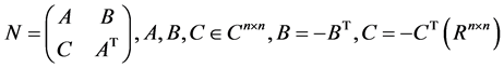
2).

As seen, in the square of the Hamiltonian matrix the angle cells B and C are asymmetric, and the diagonal ones transposed relative to each other.

If and (L_i―the eigenvalues), then

These observations determine the base of the next SR algorithm for computation of the eigenvalues L₁, L₂, ∙∙∙, L_n of:

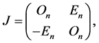
1) We define

2) We compute the unitary matrix Q, so that

,

where H is a right Hessenberg matrix

3) We use a QR algorithm for computing

.

4) For i from 1 to n we compute, taking a square root, located in the left half of the interval. In the set is fulfilled, that

Point 2 of the plan of the SR algorithm is the only action in this process, which requires immediate clarification.

We will consider one step of the algorithm by which we will show how the unitary symplect can be determined.

We will describe the original matrix, as follows:

(The zero diagonals in B and C are due to the asymmetricity). It turns out that the block C of this matrix can be zeroed by the use of a sequence of Householder and Givens symplectic similarity transformations.

The first action is to zero C₃₁ and C₄₁, using the Householder matrix, at k = 1, using working algorithm H at,. Here.

The working algorithm H in short is used for determining the vector, so that, if

, then for.

We compute.

We construct in the following way:

, for.

We construct the Householder matrix

,

where

The exchange of the locations of y and z can be used for determining the matrix H_k, so that v_i = 0, for.

It may be noticed that when the similarity transformation is executed with the first matrix, only the rows and columns 2, 3 and 4 of A, B and C affect the results:

The zeroing of positions (13) and (14) of C follows from the asymmetricity of this matrix.

The next action is to zero, using a Givens similarity transformation. This can be accomplished through the use of a working algorithm J, at which is constructed a matrix at, , k = 1.

The algorithm in brief consists of the following:

1) We compute.

2) If, then, , otherwise,

3) We construct the matrix, which has the following type:

,

where

,

.

Here the argument.

After performing the transformation can be noted that only the second row and column of A, B and C are affected by the result:

The next action of the SR algorithm is to zero a₃₁ and a₄₁ from the matrix. This can be done through the use of the working algorithm H, but with a correction at the construction of the matrix. Here now, , k = 1 and the vector W is selected in another way:

,.

The result of the transformation is the following:

It may be noted that only rows and columns 2, 3 and 4 of A, B and C are transformed from this transformation.

With this is finished the zeroing in the first column of N (at k = 1).

After steps with the working algorithm N applied respectively for the matrices A and C and steps with the working algorithm J for the matrix C, the matrix N obtains the desired look. Therefore, for the unitary matrix Q we can claim that is has the following look:

.

In conclusion of this method may be mentioned that it is used for development of the simplex method for solving algebraic and differential equations of Riccati.

3. Formalized Model for Hamiltonian Matrices

For a conditional n-qubit system, represented by the N-dimensional matrix U the input data, accepted to be |α›, to the matrix U and the output data, may be defined as

:

Since

(1)

Recently we have described a model of a formalized programmable circuit, which can be used for simulating the action of the matrix U in Equation (1) only by determining the angles of the matrix elements. The aim is to establish circuit equivalents for the rows of matrix in N × N block quantum operations; and then to combine the blocks through the use of 2ⁿ⁺¹ different states of the (n + 1) ancilla control qubits (Figure 1).

(2)

Here, each submatrix V_i have the ithe row from the given matrix as its first row in the following form. The normalization constant is. We use the symbol “•” for the elements, which are of minor importance in the overall scheme.

In order to use the matrix V instead of the matrix U in Equation (1), we modify the input data in Equation (1) to a vector φ so that φ to be carried into the elements of. Therefore, the expected results of can also be continued on some predetermined states in the results of. This is shown below:

(3)

where and are the normalization constants.

The other states in the output data represented with “•”, are subject to ignoring. Therefore, the likelihood of success of the postselection of the zero state in the main qubits, which is a success of the simulations, is given by к². For example, if N = 2, Equation (3) becomes as follows:

(4)

The separation of the main and ancilla qubits in the circuit is entirely artificial, since their roles may be exchanged in the circuit. In order to facilitate the process of verification, the circuit is divided into: Input Modification, Formation and Combination.

In the process for estimation of the phase for facilitation, we exchange the computing qubits at the end with the auxiliary qubits at the beginning and we use the following output data, instead of those of Equation (3):

(5)

where the first N states are selected to be the important states.

By measuring all ancilla qubits in a computer way and the postselection for the result, we obtain in the remaining n qubits state (as entered in Equation (1)). In this case the likelihood of success is κ² = 1/2²ⁿ.

4. Eigenfunctions of Hamiltonian Matrices

The polar form of the complex eigenvalue λ_j, belonging to the matrix U, can be written as:

(6)

where is the phase, and is the significance of the relevant eigenvalue. For the unitary matrices. Then can be applied the phase estimation algorithm to find the value of the phase and hence the eigenvalue λ_j. The circuit, shown in Figure 2, is an iterative version of the algorithm for estimation of the phase (IPEA) [6] [19] , which can also be used for estimation of the value of. Each iteration of IPEA is computed a bit of the m-digit binomial development of the phase:

(7)

the number of iterations m justify the precision. Xk is the binary value, derived from the kth iteration of the IPEA through the use of the th power of the matrix.

For the Hamiltonian matrices, however, the algorithm for estimation of the phase by itself is not enough. To compute the eigenvalue both parameters φ_j and r_j must be found. Through the use of the IPEA with the main circuit, described in the preceding section, the parameters φ_j and r_j can be found, and hence the eigenvalues of the Hamiltonian matrices can also be found by the algorithm for estimation of the phase without additional cost. Since the fixed circuit size the usage of the IPEA to the model of the circuit also has a fixed model. Therefore, we only need to set the values of the angles in each iteration of the IPEA.

4.1. Estimation of ϕ_j

In order to use the basic model of the circuit shown in Figure 3, within the IPEA, we must determine the connection between the selected states and the phase qubit obtaining in the measurement. Because there are 2n Hadamard operators in the circuit, κ = 1/N. In the estimation of the phase because all operators are controlled by an upper qubit, this scaling effect of κ is valid for the phase qubit with value one. In order to have the same scaling at phase qubit zero, we use the Hadamard operators on the ancilla qubits to act without control qubit. But when

the phase qubit is zero the controlled Hadamard operator on the ancilla qubit is used a scaling operator which operates. This operator has the following structure:

(8)

In Figure 4 is shown the resulting circuit for two qubit systems. All of the operators are controlled only the Hadamard operators on the ancilla qubits are not. For the phase qubit with a zero value, the algorithm gives this result on the remaining qubits:

(9)

where κ = 1/N. Therefore, where the ancilla is zero in the output data the phase of the selected N states can be calculated

In the evolution of the system for each loop of the algorithm for estimation of the phase, the effect of the eigenvalue can be observed in the evolution:

(10)

where, and represent the phase, ancilla and the main qubits. The eigenstate of the operator U is. After the first Hadamard operator, the result becomes:

(11)

When the, the usage of the formalized model leads to the result of the selected states. Since the Hadamard operators are not controlled, they are the only operators that operate when. Therefore, after the usage of the formalized model with operator SCALE (which scales input state, where the phase qubit is zero), we obtain the following:

(12)

where represents the formalized model in Figure 3 from the equation with eigenvalues. At the selected states stimulates U. Hence if we take into account the selected states (the states in which the ancilla qubit is), , where κ is the normalization constant. That is why we have the following wave function that describes the selected states in the first loop:

(13)

and the states that do not include, are ignored. The application of the rotation operator around the z-axis on the phase qubit in the circuit ensures that only one bit, x_k in, of the phase is estimated in each iteration. From this follows that after this operator the condition becomes e^i2π(0∙xk):

(14)

When the last Hadamard operator is applied to the phase qubit, the last state is as follows:

(15)

or in shorter form:

(16)

Here, because of the size of the system κ = 1/2. For the general case κ is directly related to the size of the ancilla qubit and is 1/n, if there are (n + 1) qubits in the ancilla. Thus, the upper equation can be presented in a general form, as follows:

(17)

Since x_k is a bit value, it can be 0 or 1. When x_k = 0, since e^i2π0 = 1, the above equation is reduced to:

(18)

In the case when x_k = 1, since e^iπ = −1, Equation (17) becomes:

(19)

Since; if x_k = 0, the probability to be found the phase qubit in state is higher than the probability to be found in. If x_k = 1, then the probability to be found the phase qubit in is higher. Thus, from the measurement of the phase qubit can be determined x_k.

In each iteration of the algorithm for estimation of the phase in this way is determined a different bit of the phase. For the κth iteration of the algorithm for estimation of the phase for determining the κth digit of the phase, we see. Hence, for the more we increase the power of U or the accuracy, the more the amplitude of the and states come closer. In this case a single iteration of the PEA may repeat the protocol several times for collection of sufficient statistical data for determining the phase bit with high confidence. This is especially important for the further iterations, where for the probability to be found the phase qubit in and is exponentially close (in к―the index of iteration).

4.2. Computing |λ_j|

As we have shown above, the phase qubit output probability, when the ancilla is zero, is determined by. We measure or with probability P, equal to. Hence, we obtain

(20)

Since κ and P are known (for matrix 2 × 2 the value of κ is 1/2 because both Hadamard operators in the circuit), can be determined from the measurement statistics. Therefore, the accuracy of the estimated value of can further be improved by the use of all iterations of the algorithm for estimation of the phase: for the κth iteration, as a general form, is obtained the following:

(21)

By taking the average estimates from different iterations of the estimation of the phase, the estimate of can become more accurate. In conclusion, through the use of and ϕ_j in Equation (6) we can compute the eigenvalue of the Hamiltonian matrix.

5. Discussion

In order to generate the matrix elements through the use of rotation operators around the y- and z-axis, in the algorithm for estimation of the phase the absolute values of the elements must be less than one. One of the ways to achieve this is to separate all the elements by the maximum element absolute value. This ensures that on the basis of the relationship of the norm and the eigenvalue, the largest absolute eigenvalue is less than the absolute sum of the row or the column of the matrix, which can be maximum N (i.e. since the absolute maximum value is 1). It is not recommended the eigenvalue to be less than one. If the eigenvalues, however, are larger than 1, this approach may require scaling within the very algorithmiteration, since in the powers there is a possibility the elements to become again greater than one. Another approach to be scaled the elements is to be used the first norm or the infinite norm of the matrix, which are easy for computing. The scaling of the matrix through the norm makes the eigenvalue less than 1, and thus in the matrix power the elements go towards zero. Hereinafter the scaling is done only at the beginning. Therefore in the κth iteration in the algorithm for estimation of the phase we have, where µ is the scaling, used at the beginning. Hence, if without scaling, the more we increase the power of U or the accuracy, the more the amplitude of the states and come closer. For after several iterations it becomes difficultly applicable to distinguish whether the phase qubit is 0 or 1. The scaling of the powers of U, which generates the eigenvalue, can be used to remedy this problem.

The accuracy for determining the value of r_j requires to be determined the states (1 + r_j) and (1 − r_j) in the probabilities for finding the phase qubit in or from the statistical data of the measurements. The accuracy in these statics is different on the basis of the measurement protocol, the quantum state, the basic quantum machine and even the amount of quantum entanglements [13] [14] .

Complexity of the Algorithm

The complexity of the algorithm for estimation of the phase with one iteration is dominated mainly by the complexity of the implementation of the given operator. It is also necessary to be made a tomography of the state of the phase qubit, in order to be determined the absolute eigenvalue, which is different on the basis of the basic quantum machine used in the algorithm for estimation of the phase.

It is known that the complexity of implementation of the operator of the quantum computer requires O(N²) number of operations with one and two qubits. In addition, more effective circuits are possible for the sparse matrices. The general matrix, described in Figure 3, also follows the same characteristic of complexity for a detailed analysis of the complexity of the circuit). In the circuit exists a quantum network composed of N² rotation operators, constantly controlled by the first 2n qubits. The decomposition of this network requires 2²ⁿ number of CNOTs and 2²ⁿ single rotation operations, which are explained in Annex B. Hence, the circuit in total requires 2²ⁿ CNOT, 2²ⁿ single rotation, 2n Hadamard and n SWAP operators. And so the overall complexity is O(N²). Please also note that for the zero elements there is no need to be used rotation operators. Thus for the sparse matrices the operations number can be reduced.

Because the complexity of one iteration of the algorithm for estimation of the phase is dominated by the complexity of the implementation of a given operator, each algorithm iteration requires O(N²) operations. Then, for m number of iterations we obtain O(mN²) as the complexity.

When the powers of the matrix cannot be effectively computed, the complexity for computing the power of matrix U at classical computers must also be taken into account. The power of the matrix may be found by using the method of successive squaring, which requires only one dot matrix multiplication. Then the total complexity becomes a combination of these two:

(22)

where m is the number of the iterations, M is the complexity of the matrix multiplication. Note that, even if it is necessary the powers of the matrix to be computed, at least this is still at least as effective, as the classical algorithms, which require to a great extent O(N3) time for finding an eigenvalue. Also note that the complexity of the algorithm in Equation (22) does not include the complexity of measurement and determination of the value of r_j. It depends on the measurement protocol, the quantum state and the basic quantum machine. Additionally, the total number of iterations m can be large in cases in which, for, the probability of finding the phase qubit in or states becomes exponentially (in the index of iteration κ) close, since the single iteration of the PEA may require repetition of the protocol several times for collecting sufficient statistical data for determining the phase bit with high confidence.

In comparison with the work done by Wang et al., the likelihood of success decreases exponentially in both algorithms described in this report and in their report. In our case, however, by scaling the matrix elements in each iteration of the algorithm, the likelihood can be increased. Moreover, here we can find the values of the angles for the rotation operators very easily for implementation of the given operator. However, in their method, the subsystems H_A and H_B and their interaction H_AB must be found in order to be implemented the given H: H = H_A + H_B + H_AB. In terms of the quantum complexity, because their method is based on Hamiltonian successive projective measurements on H_A, which cannot be implemented deterministically, the complexity exponentially increases. Put in other words, in their case the finding of the given operator powers is easier, but when the size of the subsystem H_A is large, the complexity is dominated by the complexity of the measurements.

6. Application to Non-Hermitian Quantum Systems

Certain tasks can be extremely difficult or even impossible to be solved within the standard formalism of the quantum mechanics, where the obvious properties of the dynamic nature are real and are associated with the eigenvalues of the Hermitian operators. In most implementations of the standard quantum Hermitian formalism the use of a Hermitian operator is presented as an equivalent to a non-Hermitian operator. The phenomena resonance, in which the particles are temporarily caught by the potential, can be examined in the scope of the non-Hermitian quantum mechanics. In the non-Hermitian quantum mechanics the resonant states’ lifetime is proportionally dependent of the behavior of the imaginary part of the eigenvalue. Let’s suppose that we have a non-unitary operator U = e^−iHt/ħ for a non-Hermitian Hamiltonian H with eigenstates of the energy and the corresponding energy eigenvalues E_j, i.e.. Since E_j is an eigenvalue of H; if t and ħ are set to 1, then is the eigenvalue of U. Therefore a N × N non-unitary transformation U possesses eigenvectors with corresponding eigenvalues. As shown in Sec. 3, the eigenvalue λ_j of the matrix U can be evaluated. This also allows us to define the respective eigenvalue E_j of the Hamiltonian H from. Note that in our procedure for phase estimation, because the elements of the matrix are used directly in the circuit, we can also use directly the matrix of Hamiltonian H, in lieu of U.

Conclusion

We have presented a basic scheme for the execution of an algorithm for phase estimation for matrices of Hamiltonian (Appendix). Because the circuit model for matrices of Hamiltonian represents a basic programmable circuit, the circuit for the phase estimation algorithm is also formalized: it may be used for each matrices type for computing its eigenvalues. We showed that the complex eigenvalues of the non-Hermitian quantum systems may be found by means of this method. As an example we have shown how the resonant states of a model of the Hamiltonian are examined.

Cite this paper

NikolayRaychev, (2016) Formalized Quantum Model for Solving the Eigenfunctions. Journal of Quantum Information Science,06,16-30. doi: 10.4236/jqis.2016.61003

References

Appendix

By way of example, we look at the next radial Hamiltonian:

(23)

wherever J and a are free potential parameters (J is the potential depth in the potentialgraph. a is associated with the potential barrierwidth.) The potential element in the upper Hamiltonian indicates the predissociation resonances that are quasibound states referring to the eigenvalues complex part. To illustrate, using just a two basic functions, orthonormal eigenfunctions of an harmonic oscillator, where the mass is equal to one and the frequency is equal to a) and the setting J = 0.1 and a = 0.1; The matrix of Hamiltonian is calculated as [18] :

(24)

which has its own eigenvector:

(25)

and the basic state eigenenergy (0.6249 − 0.4139i). Because the upper matrix of Hamiltonian is non-Hermitian, the time evolution operator, found from U = e^−iHt/ħ, is non-unitary, and is calculated as:

(26)

with the eigenvalue 1.2268 + 0.8849i. We used the above-described phase estimation method, to simulate this non-unitary operator and to determine the complex eigenvalues of H. In the simulation, because the matrix elements absolute values of U are greater than 1, we scale the elements by means of the first matrix norm. This causes the elements of the matrix of U to proceed towards zero in the limit. We use 11 iterations in the phase estimation algorithm. After the 11th iteration the probability difference between seeing the phase qubitas 0 or 1 is almost equal.

Therefore, from the simulation results, we calculate the eigenvalue of U as 1.22255 + 0.88355i, and thereby also the eigenvalue of H as 0.6259 − 0.4089i, which gives an error in the series of 10⁻³. This iscoming from the error of rounding and the limited available powers of U (when the power proceed towards zero, we can no longer distinguish and of the phase qubit; the probabilities are becoming equal).

References

- 1. Rebentrost, P., Mohseni, M., Kassal, I., Lloyd, S. and Aspuru-Guzik, A. (2009) Environment-Assisted Quantum Transport. New Journal of Physics, 11, 033003.
http://dx.doi.org/10.1088/1367-2630/11/3/033003 - 2. Rebentrost, P., Mohseni, M. and Aspuru-Guzik, A. (2009) Role of Quantum Coherence and Environmental Fluctuations in Chromophoric Energy Transport. The Journal of Physical Chemistry B, 113, 9942-9947.
http://dx.doi.org/10.1021/jp901724d - 3. Ishizaki, A. and Fleming, G.R. (2009) Unified Treatment of Quantum Coherent and Incoherent Hopping Dynamics in Electronic Energy Transfer: Reduced Hierarchy Equation Approach. The Journal of Chemical Physics, 130, 234111.
http://dx.doi.org/10.1063/1.3155372 - 4. Ishizaki, A. and Fleming, G.R. (2009) Theoretical Examination of Quantum Coherence in a Photosynthetic System at Physiological Temperature. Proceedings of the National Academy of Sciences of the United States of America, 106, 17255-17260.
http://dx.doi.org/10.1073/pnas.0908989106 - 5. Raychev, N. (2015) Quantum Algorithm for Spectral Diffraction of Probability Distributions. International Journal of Scientific and Engineering Research, 6, 1346-1349.
http://dx.doi.org/10.14299/ijser.2015.07.005 - 6. Raychev, N. (2015) Algorithm for Switching 4-Bit Packages in Full Quantum Network with Multiple Network Nodes. International Journal of Scientific and Engineering Research, 6,1289-1294.
http://dx.doi.org/10.14299/ijser.2015.08.004 - 7. Reed, M.D., DiCarlo, L., Johnson, B.R., Sun, L., Schuster, D.I., Frunzio, L. and Schoelkopf, R.J. (2010) High Fidelity Readout in Circuit Quantum Electrodynamics Using the Jaynes-Cummings nonlinearity. Physical Review Letters, 105, 173601.
- 8. Strauch, F.W., Johnson, P.R., Dragt, A.J., Lobb, C.J., Anderson, J.R. and Wellstood, F.C. (2003) Quantum Logic Gates for Coupled Superconducting Phase Qubits. Physical Review Letters, 91, 167005.
http://dx.doi.org/10.1103/PhysRevLett.91.167005 - 9. Raychev, N. (2015) Reply to “The Classical-Quantum Boundary For correlations: Discord and Related Measures”. Abstract and Applied Analysis, 94, 1455-1465.
- 10. Feynman, R.P. (1982) Simulating Physics with Computers. International Journal of Theoretical Physics, 21, 467-488.
- 11. Raychev, N. (2015) Mathematical Approaches for Modified Quantum Calculation. International Journal of Scientific and Engineering Research, 6, 1302-1309.
http://dx.doi.org/10.14299/ijser.2015.08.006 - 12. Sorensen, S., Demler, E. and Lukin, M.D. (2005) Fractional Quantum Hall States of Atoms in Optical Lattices. Physical Review Letters, 94, 086803.
http://dx.doi.org/10.1103/PhysRevLett.94.086803 - 13. Lim, L.-K., Morais Smith, C. and Hemmerich, A. (2008) Staggered-Vortex Superfluid of Ultracold Bosons in an Optical Lattice. Physical Review Letters, 100, 130402.
http://dx.doi.org/10.1103/PhysRevLett.100.130402 - 14. Hemmerich, A. (2010) Effective Time-Independent Description of Optical Lattices with Periodic Driving. Physical Review Letters, 81, 063626.
http://dx.doi.org/10.1103/PhysRevA.81.063626 - 15. Eckardt, A., Hauke, P., Soltan-Panahi, P., Becker, C., Sengstock, K. and Lewenstein, M. (2010) Frustrated Quantum Anti-Ferromagnetism with Ultracold Bosons in a Triangular Lattice. Europhysics Letters, 89, 10010.
http://dx.doi.org/10.1209/0295-5075/89/10010 - 16. Creffield, C.E. and Sols, F. (2011) Directed Transport in Driven Optical Lattices by Gauge Generation. Physical Review A, 84, 023630.
http://dx.doi.org/10.1103/PhysRevA.84.023630 - 17. Miyake, H., Siviloglou, G.A., Kennedy, C.J., Burton, W.C. and Ketterle, W. (2013) Realizing the Harper Hamiltonian with Laser-Assisted Tunneling in Optical Lattices. Physical Review Letters, 111, 185302.
http://dx.doi.org/10.1103/PhysRevLett.111.185302 - 18. Aidelsburger, M., Lohse, M., Schweizer, C., Atala, M., Barreiro, J.T., Nascimbene, S., Cooper, N.R., Bloch, I. and Goldman, N. (2014) Revealing the Topology of Hofstadter Bands with Ultracold Bosonic Atoms.
http://arxiv.org/abs/1407.4205v1 - 19. Raychev, N. (2015) Quantum Computing Models for Algebraic Applications. International Journal of Scientific and Engineering Research, 6,1281-1288.
http://dx.doi.org/10.14299/ijser.2015.08.003 - 20. Toth, G. and Guhne, O. (2005) Entanglement Detection in the Stabilizer Formalism. Physical Review A, 72, 022340.
http://dx.doi.org/10.1103/PhysRevA.72.022340 - 21. Raychev, N. (2015) Indexed Cluster of Controlled Computational Operators. International Journal of Scientific and Engineering Research, 6, 1295-1301.
http://dx.doi.org/10.14299/ijser.2015.08.005 - 22. Raychev, N. (2015) Quantum Multidimensional Operators with Many Controls. International Journal of Scientific and Engineering Research, 6, 1310-1317.
http://dx.doi.org/10.14299/ijser.2015.08.007 - 23. Veis, L. and Pittner, J. (2010) Quantum Computing Applied to Calculations of Molecular Energies: CH2 Benchmark. The Journal of Chemical Physics, 133, 194106.
http://dx.doi.org/10.1063/1.3503767