Journal of Geographic Information System
Vol.6 No.2(2014), Article ID:44565,11 pages DOI:10.4236/jgis.2014.62010
Quantitative Methods for Comparing Different Polyline Stream Network Models
Danny L. Anderson1, Daniel P. Ames2, Ping Yang3
1Idaho National Laboratory, Idaho Falls, USA
2Department of Civil and Environmental Engineering, Brigham Young University, Provo, USA
3Texas Institute for Applied Environmental Research, Tarleton State University, Stephenville, USA
Email: dan.ames@byu.edu
Copyright © 2014 by authors and Scientific Research Publishing Inc.
This work is licensed under the Creative Commons Attribution International License (CC BY).
http://creativecommons.org/licenses/by/4.0/


Received 20 February 2014; revised 20 March 2014; accepted 27 March 2014
ABSTRACT
Two techniques for exploring relative horizontal accuracy of complex linear spatial features are described and sample source code (pseudo code) is presented for this purpose. The first technique, relative sinuosity, is presented as a measure of the complexity or detail of a polyline network in comparison to a reference network. We term the second technique longitudinal root mean squared error (LRMSE) and present it as a means for quantitatively assessing the horizontal variance between two polyline data sets representing digitized (reference) and derived stream and river networks. Both relative sinuosity and LRMSE are shown to be suitable measures of horizontal stream network accuracy for assessing quality and variation in linear features. Both techniques have been used in two recent investigations involving extraction of hydrographic features from LiDAR elevation data. One confirmed that, with the greatly increased resolution of LiDAR data, smaller cell sizes yielded better stream network delineations, based on sinuosity and LRMSE, when using LiDAR-derived DEMs. The other demonstrated a new method of delineating stream channels directly from LiDAR point clouds, without the intermediate step of deriving a DEM, showing that the direct delineation from LiDAR point clouds yielded an excellent and much better match, as indicated by the LRMSE.
Keywords:LiDAR, Stream Channels, Accuracy, RMSE, Sinuosity, Terrain Analysis

1. Introduction
All spatial data are of limited accuracy [1] . However, if we assume one dataset to be the best available representation of a particular feature, then we can estimate the error contained within other features by comparing them to our reference data. In some cases, it may not be critical that the modeled or derived dataset perfectly matches the reference dataset, as long as it is a better match than is another dataset. According to Zhang and Goodchild [2] [When considering] the acquisition of discrete objects by visual interpretation and manual delineation, an extracted (measured) object is different from the corresponding truth due to inaccuracy in object identification and positioning... In most discrete representations, real-world line objects are sampled by polylines that link up ordered vertices with straight line segments. If the real lines are truly curved, ... a polyline representation will be an approximation, and such differences between polylines and the original curves form part of the uncertainty in modeling objects.
While it is trivial to compare a set of scalar values (with a single magnitude) or a set of vectors (with a magnitude and direction), it is more challenging to compare and assess the degree of similarity of sets of polylines. More difficult, still, is the comparison of networks of numerous sets of polylines. For example, in Figure 1, red polylines represent a derived stream network and the blue polylines represent the reference stream network. We can clearly see that the two networks are not identical. But, how do we quantify the differences to compare the quality or similarity of the two networks, or to compare multiple derived networks with each other, relative to the reference network? This paper presents and evaluates two methods and algorithms for performing quantitative comparisons of the closeness of fit between derived stream networks and reference data: sinuosity and Longitudinal Root Mean Square Error (LRMSE).
2. Background
Accuracy assessment or validation of feature data accuracy should be a key component of any project employing spatial data. This is particularly necessary when modeling or otherwise automatically generating spatial data from computational algorithms or methods (e.g. in the case of the derived stream networks in this study). Such an assessment of accuracy allows one the ability to quantitatively compare methods and results, explore methods for improving techniques and algorithms, and be more confident in the use of spatial data analysis results in decision-making processes [3] .
Hydrological modeling and watershed resource management require accurate stream networks and watershed boundaries for better understanding the flow of water on the land surface. Methods for deriving detailed hydrographic features such as stream networks have been greatly improved in moving from conventional DEMs [4] -[6] to LiDAR-derived DEMs [7] . Quantitative assessment methods can be used to compare and analyze the differences between stream networks and watersheds derived from elevation data using such methods.
Stream channel sinuosity has been defined as the degree to which a river channel departs from a straight line. A variety of sinuosity indices have been proposed [8] -[14] . Sinuosity was employed to improve understanding
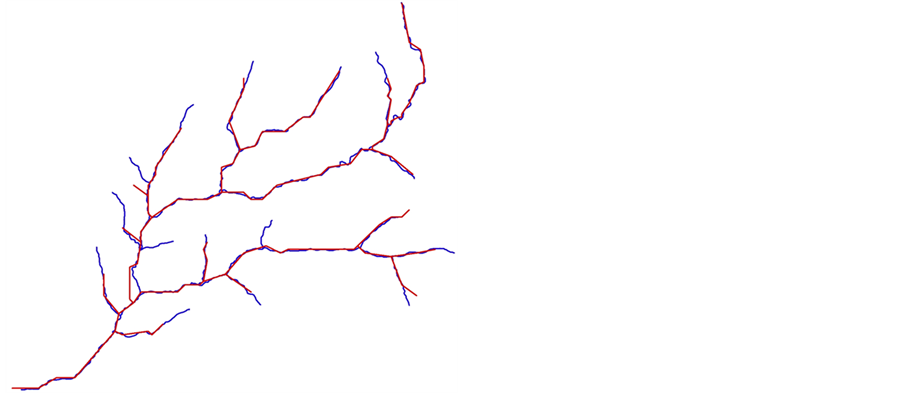
Figure 1. Two polyline representations of the same stream network with the reference network shown in blue and the derived stream network shown in red.
of the nature and dynamics of river channel patterns for the river Elemi in southwestern Nigeria, in which the length of a reach was measured along the channel and divided by the airline distance between the two end points of the reach [15] . Factors influencing sinuosity were identified for the Pannagon River, India [16] . Downward, Gurnell, and Brookes [17] presented a methodology for quantifying river channel planform change using GIS variability in stream erosion and sediment transport. Heo et al. [18] studied the meandering channel migration of the Sabine River in the USA, which proved least squares estimation is beneficial for characterization and prediction of meandering channel migration.
Work has been done on stream network assessment using root mean square error both in horizontal and vertical measurements, which have been adopted as standard methods by the Federal Geographic Data Committee [19] . Zhang and Goodchild [2] also discuss using RMSE as a measure of errors in continuous variables associated with spatial data.
Both of these assessment criteria, sinuosity and RMSE, are further explored in this paper as candidates for quantitatively assessing the quality of LiDAR-derived stream networks. Algorithms to implement these methods have been developed and scripts or program codes have been written and used to support two reported investigations [7] [20] .
3. Methods
The accuracy assessment of a stream network such as the one shown in Figure 1, involves the repeated calculations of the distance between two points. There are 33 polyline segments in the network shown. Each polyline segment is composed of numerous straight-line segments. Each straight-line segment is defined by two points (or vertices), and each point (or vertex) is defined by two coordinates (an ordered pair). The complexity of performing data quality assessments on this network is very evident. Additionally, the coordinates (vertices) could exist in any of a large number of coordinate systems, based on map projections. GIS and associated programming languages are suitable for dealing with all of the coordinate systems and for converting coordinates between the systems allowing for assessment of stream networks accuracy in any projected (e.g., Universal Transverse Mercator—UTM) or geographic (latitude and longitude) coordinate system.
The sinuosity and LRMSE methods described below require computation of distances between two points. Such a computation is trivial in the case of projections that are essentially Cartesian coordinate system (X, Y), where X is the Easting, and Y is the Northing. Here, distance between two points can be calculated using the distance equation that is based on Pythagorean’s Theorem:
 (1)
(1)
In the case of computation of distances between points represented in geographic coordinate systems, one must work with spherical coordinates (r, q, j), where r is the radius of the earth Re at a particular latitude q and longitude j. On very small scales and for comparison purposes, one can compute distances in terms of decimal degrees by applying the common distance equation (Equation (1)) to the geographic coordinate system. However, a more accurate calculation of distance between two points in geographic coordinates is the Great Circle Arc equation, which, assuming an approximately constant earth radius Re, is:
 (2)
(2)
Optimally, these and related equations are used within a GIS and its associated programming language to perform distance calculations using embedded native functions, wherever possible. Such computational environments also offer inherent ability to treat polyline constructions as objects in code and to rapidly and easily perform mathematical operations, such as distance calculations, on multiple polyline features or objects, in multiple data layers, representing large complex networks of stream channels, in any of a number of projections or coordinate systems. Pseudo codes for the algorithms we have developed and implemented in GIS are provided in the following sections. While our complete application of the algorithms was done within the ArcView 3.2 Avenue scripting environment, our pseudo code representations are software-agnostic, though we do assume the existence of specific and common GIS functions for performing complex calculations on geographic features. The algorithms presented here can be implemented in any GIS programming environment or any other suitable tool or programming language, as long as special routines exist or are developed to handle the point and polyline objects that constitute the stream network representations.
3.1. Sinuosity
Sinuosity is used to describe the condition of being winding or curving in shape and is used here as a quantitative index of stream meandering and as a distinctive property of channel pattern. Stream sinuosity is often used in the study of the geometry, dynamics, and dimensions of alluvial channels [13] . The absolute value of sinuosity differences between the reference and the derived samples can be used as a measure of modeled network accuracy.
Sinuosity (S) is the ratio of stream length to valley length [21] or, in other words, the ratio of stream length to the straight-line distance between end-points. This is also known as the degree of meandering [22] , or the ratio of the meandering length (Lm) to the straight-line distance (Ls).
 (3)
(3)
Calculating the straight-line distance between two points is simple enough in any computer code using the common distance equation, given as Equation (1) above. But, to calculate the curvilinear distance or length, this equation must be used repeatedly, once for each line segment in the polyline. This is where GIS programming languages have an advantage over non-GIS programming languages. The ability to treat a point or a polyline as an object and operate on it using pre-defined methods created specifically for dealing with geospatial features makes the calculation of the curvilinear distance or length a trivial matter. Also, GIS programming languages simplify repeating the process for multiple polylines all in the same data layer and eliminate the need for complicated input/output (I/O) routines to read and write results. The algorithm presented here assumes that a polyline data layer is selected. The algorithm cycles through each polyline in the data layer and calculates the curvilinear or meandering length, Lm, as the variable CalfPath, using an appropriate GIS polyline Length function (e.g., the Avenue ReturnLength method). Then, it calculates the direct-line distance, Ls, between the two endpoints, as the variable CrowFlies, using an appropriate GIS Distance function (e.g., the Avenue Distance method). Sinuosity is then calculated by dividing CalfPath by CrowFlies. These three values are added to the data layer’s attribute table in three new fields. The algorithm also maintains a running sum of the lengths of all features, calculates the average polyline length and the average sinuosity, and reports these values when the algorithm is finished. The algorithm is summarized as pseudo code in Table 1.
The basis for using sinuosity is an assumption that, in general, higher sinuosity implies greater detail and, therefore, greater accuracy (see Figure 2). However, the goal is not to maximize sinuosity, but rather obtain the closest possible match of sinuosity between the derived stream network and the reference stream network. If the sinuosity of the derived data is lower than that of the reference data, then less detail and, hence, less accuracy can be inferred. However, if the sinuosity of the derived data is higher than that of the reference data, we can infer greater detail, but not necessarily greater accuracy. Indeed, higher sinuosity in the derived data could just mean that the derivation process, in this case stream channel delineation, failed.
Sinuosity for two polylines can be directly compared, or relative sinuosities can be calculated. Relative sinuosity could be a delta or difference, such as
 (4)
(4)
Or relative sinuosity could be a ratio (derived sinuosity/reference sinuosity or vice versa), such as,
 (5)
(5)
One possible pitfall in using sinuosity to compare streams or networks of streams is the result of using ratios (S = Lm/Ls and Srel = Sd/Sr). Although the sinuosity of both the derived streams and the reference streams may closely match, it is possible to have closely matched sinuosities and yet have the derived stream be half the length of the reference stream. The ratio of Lm to Ls may be the same for both derived and reference streams, because both Lm to Ls are shortened proportionally. One must also examine and compare straight-line stream lengths; the distance between the endpoints should be similar. The derived stream will likely have a shorter straight-line length, but it should not be significantly shorter. Matching sinuosities does not necessarily imply that the polylines match; only that they have similar amounts of meandering. Some subjective interpretation of the objective data is still needed.

Table 1. Pseudo code for calculating sinuosity.
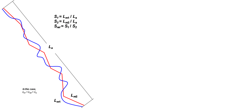
Figure 2. Sinuosity (straight-line distance vs. meandering length) as one measure of detail and closeness of fit between derived and reference stream networks.
3.2. Longitudinal Root Mean Square Error
The second metric for comparing stream networks is Longitudinal Root Mean Square Error (LRMSE). The National Standard for Spatial Data Accuracy (NSSDA, 1998) uses root-mean-square error (RMSE) to estimate positional accuracy. RMSE is the square root of the average of the set of squared differences between dataset coordinate values and coordinate values from an independent source of higher accuracy for identical points. Positional errors, also known as displacements or distortions, are understood as the differences between the measured and the assumed true coordinates.
Zhang and Goodchild [2] suggest that “metrics of root-mean-square error (RMSE) are useful indices of errors in continuous variables.” Referencing the American Society for Photogrammetry and Remote Sensing, they state that…
an empirical, site-specific estimate of positional uncertainties can be produced via tests against an independent source of much higher accuracy (this somewhat circular approach is necessary because no reference source can have perfect accuracy). Depending on the specific requirements, the independent source of higher accuracy may be obtained through land surveying or derived from aerial photography.
For n points with errors ei (i = 1, 2,···,n), observed as the differences in coordinates between the data sets to be tested and the more accurate reference data, the RMSE is
 (6)
(6)
where the error ei is the distance between a test or modeled data point (Xi, Yi) and a corresponding reference data point (Xoi, Yoi). In other words, for Cartesian coordinates,
 (7)
(7)
We define LRMSE as the horizontal root mean square error (RMSE) computed between a number of paired sets of points located along both derived and reference stream network polylines. Thus,
 (8)
(8)
Our algorithm for deriving LRMSE assumes that two polyline data sets are selected within the GIS environment: one would be the derived stream network and the other would be the reference stream network. For each polyline in the reference data, the reference polyline is divided into m equal-length segments between n evenly spaced points, where m = n – 1. Then, for each reference point, the nearest point on the derived polyline is identified and the distance (di) from that point on the derived polyline to the current point on the reference polyline is calculated (see Figure 3). LRMSE is then calculated as
 (9)
(9)
with m = 100 and n = 101 for our sample data.
The LRMSE values are stored in a new attribute table. If a stream branch in the reference network is missing in the derived network, then the LRMSE is reported as −9999.99. The algorithm is summarized as pseudo code in Table 2.
LRMSE is used as a measure of how accurately the derived stream networks match the reference networks. The smaller the LRMSE, the closer the fit between derived and reference data. Unlike relative sinuosity, where the goal is to closely match the calculated value for the derived network with the calculated value for the reference network, rather than maximizing the value, the goal with LRMSE is to minimize the value, since the comparison with the reference is built into the calculation.
Like the sinuosity technique, however, the LRMSE technique also has a possible pitfall. Two polylines may match up perfectly up to a point, but one polyline may be shorter, indicating perhaps that there was a failure to delineate the full reach of a stream. Ideally, because the LRMSE technique compares nearest points on the polylines, the LRMSE would be a low value indicating a close match for the common reach. But it would give no
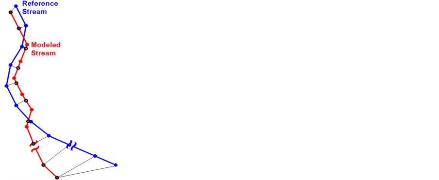
Figure 3. Computation of LRMSE between derived stream and reference stream.
Table 2. Pseudo code for calculating LRMSE.
indication that one polyline is longer than the other. As implemented, however, because the reference polyline is segmented for comparison against the derived polyline, if the reference polyline is much longer than the derived polyline, all points on the reference polyline that are beyond the end of the derived polyline will be compared with the derived polyline’s endpoint, with increasing separation distances and an increasing LRMSE. Considering this, it may be better to determine which polyline has the shorter curvilinear length and segment that polyline, comparing it with the longer polyline. In this case, the extension of the longer polyline would be ignored and LRMSE would truly indicate a good match, with the exception of extension. Such a change to the code is recommended, but has not yet been implemented and tested. Another solution, which has been used [20] , is to manually truncate the longer polyline so that only the common reach is used for comparing the two polylines. Like sinuosity, when using LRMSE, some subjective interpretation of the objective data is still needed.
3.3. Special Considerations
There are several considerations that must be made in using these methods with polylines particularly when implemented in the ArcView environment using polyline (typically “shapefile”) formatted data. First, the polylines need to “flow” in the same direction. This means that two polylines, in different stream networks that are being compared, must be constructed in the same order, upstream end to downstream end. The “flow” direction of the polylines can be checked and, if necessary, reversed, using the Line Direction Tool, developed by Jennesse Enterprises (www.jennessent.com).
If the “flow” direction must be changed, the second consideration becomes relevant. If the stream network polyline data contain “ArcZ” lines, then they need to be converted to standard polylines, because “ArcZ” lines are generally not editable. This can be easily accomplished using an Avenue script called PolyShape.Coverter, developed by Deshpande (2000).
Finally, the third consideration is that the polylines need a visual quality check to ensure that there is a one-to-one correspondence between polyline segments. This does not mean that there has to be a polyline in the derived stream network for every polyline in the reference file. If the derived polyline is missing a polyline segment, then the reference segment is ignored. However, corresponding segments in the reference and derived polyline networks must have the same identification number (ID). For example, in two of the three stream network geographic areas studied by Yang et al. (2010), discussed in the next section, the number of polylines in the reference network equaled the number of polylines in the derived network, regardless of the coarseness of the delineation, and corresponding polyline segments were assigned matching IDs. However, for coarser delineations in the third geographic area, the number of polylines differed between the reference and derived networks. One or two branches were not created in the delineation process. Where the branches were missing, the delineation process failed to create separate polylines on either side of the branch, resulting in a single long polyline in the derived network that was represented by two shorter polylines in the reference network. This longer derived polyline was then automatically compared with either of the two shorter reference polylines or to the missing branch in the reference network, depending on which of the three reference ID numbers was assigned to the derived polyline, which skewed the analyses.
To resolve this, the longer derived polylines were manually broken at about the location of the missing branches, and the IDs for the polylines in the derived dataset were changed to ensure matches between corresponding reference and derived polylines, so that derived polylines were correctly compared with the corresponding reference polylines (see Figure 4).
The accuracy assessment of a stream network such as the one shown in Figure 1, involves the repeated calculations of the distance between two points. There are 33 polyline segments in the network shown. Each polyline segment is composed of numerous straight-line segments. Each straight-line segment is defined by two points (or vertices), and each point (or vertex) is defined by two coordinates (an ordered pair). The complexity of performing data quality assessments on this network is very evident. Additionally, the coordinates (vertices) could exist in any of a large number of coordinate systems, based on map projections. GIS and associated programming languages are suitable for dealing with all of the coordinate systems and for converting coordinates between the systems allowing for assessment of stream networks accuracy in any projected (e.g., Universal Transverse Mercator—UTM) or geographic (latitude and longitude) coordinate system.
4. Application and Results
The relative sinuosity and LRMSE algorithms presented here were used to compare and assess the quality of a number of LiDAR-derived streams and stream networks. Yang et al. (2010) used the techniques to compare stream channel networks delineated from LiDAR-derived Digital Elevation Models for the Dry Creek, Slate Creek, and Reynolds Creek watersheds, in Idaho, USA. Figure 5 shows the average sinuosity for the three study areas. Figure 6 shows the ratios of derived (or sample) sinuosity to reference sinuosity for the three study areas.
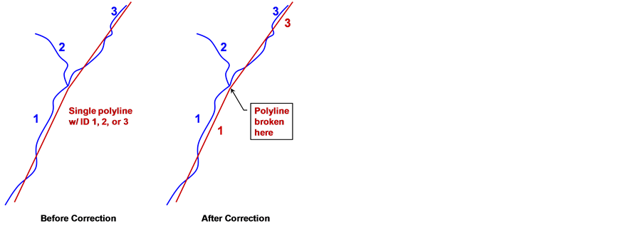
Figure 4. Manually breaking polylines to ensure one-to-one correspondence.
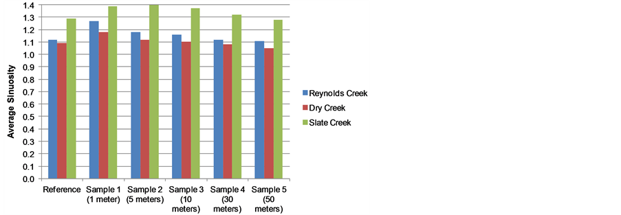
Figure 5. Average sinuosity for stream networks delineated from LiDAR-derived DEMs.
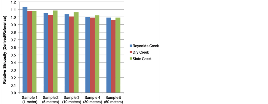
Figure 6.Relative sinuosity (derived/reference) for stream networks delineated from LiDAR-derived DEMs.
A value of 1.0 indicates a perfect match in sinuosity, although not necessarily a perfect overlying match of polylines. Note that, for Reynolds Creek, the 30-meter cell size yields a sinuosity that most closely matches the reference; for Dry Creek, the 10-meter cell size yields a sinuosity that most closely matches the reference; and for Slate Creek, the 50-meter cell size yields a sinuosity that most closely matches the reference.
Figure 7 shows the average LRMSE for derived stream networks versus reference stream networks for the three study areas. Note that, generally, the LRMSE decreases (indicating better match) as the cell size decreases. Further discussion of these results can be found in Yang et al. (2010).
Anderson and Ames (2010) used the sinuosity and LRMSE techniques to assess a new stream network delineation method that works directly from LiDAR point cloud data, for the Fishhook Creek Inlet of Redfish Lake, in Custer County, Idaho. In this case, the LiDAR delineation was compared with a traditional DEM-based grid cell stream network delineation, two standard stream datasets, and a highly detailed reference stream traced from 1-meter resolution National Agricultural Imaging Project or NAIP aerial photography (see Table 3). Note that, while LRMSE indicates that the LiDAR point cloud delineation yielded a much better match to the reference, the DEM-based delineation yielded a relative sinuosity that most closely matched that of the reference. This supports the caution, offered in Section 3.1, that matching sinuosities do not necessarily mean that the polylines match; only that the amount of meandering is similar. LRMSE is the better of the two metrics for determining match. Although the reference and derived polylines differed in length, the longer polylines were manually truncated for fair comparison of the common reach.
5. Conclusion
Networks of polylines can be compared for relative accuracy in terms of sinuosity and LRMSE, to provide quantitative assessment of the quality of the data. Neither sinuosity nor LRMSE should be used blindly; both require some subjective interpretation to ensure that they are used properly and that there are no data anomalies, such as greatly disparate polyline lengths. Nevertheless, using these techniques for comparing polylines or networks of polyline, one can explore detailed comparisons of stream channel delineations that differ, for example, in the assumptions applied or the derivation processes employed. While LRMSE appears to be a more generally suitable technique, both provide valuable insights when properly used and reviewed. Both techniques have been
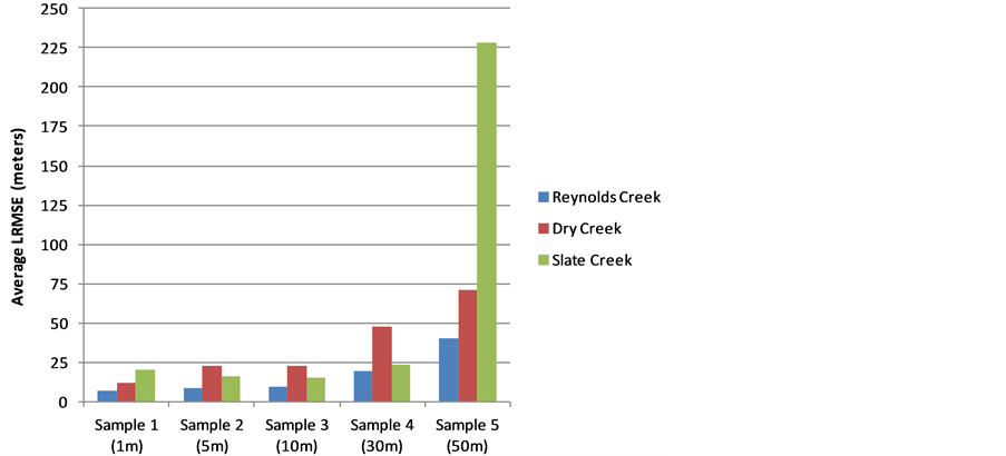
Figure 7. LRMSE for LiDAR-derived DEMs.
Table 3. Example of sinuosity and LRMSE results (Fishhook Creek).
*Relative to the NAIP Reference.
used in two recent investigations involving extracting of hydrographic features from LiDAR elevation data. In one, it is confirmed that, with the greatly increased resolution of LiDAR data, smaller cell sizes yielded better stream network delineations based on sinuosity and LRMSE when using LiDAR-derived DEMs [7] . The other demonstrated a new method of delineating stream channels directly from LiDAR point clouds [20] , without the intermediate step of deriving a DEM. It was shown that the direct delineation from LiDAR point clouds yielded an excellent and much better match, as indicated by the LRMSE.
References
- Goodchild, M.F. and Gopal, S. (1989) The Accuracy of Spatial Databases. CRC Press, Boca Raton.
- Zhang, J. and Goodchild, M.F. (2002) Uncertainty in Geographical Information. CRC Press, Boca Raton. http://dx.doi.org/10.4324/9780203471326
- Congalton, R.G. (2001) Accuracy Assessment and Validation of Remotely Sensed and Other Spatial Information. International Journal of Wildland Fire, 10, 321-328.
- Jenson, S. and Domingue, J. (1988) Extracting Topographic Structure from Digital Elevation Data for Geographic Information System Analysis. Photogrammetric Engineering and Remote Sensing, 54, 1593-1600.
- Tarboton, D.G., Bras, R.L. and Rodriguez-Iturbe, I. (1991) On the Extraction of Channel Networks from Digital Elevation Data. Hydrological Processes, 5, 81-100. http://dx.doi.org/10.1002/hyp.3360050107
- Olivera, F. (2001) Extracting Hydrologic Information from Spatial Data for HMS Modeling. Journal of Hydrologic Engineering, 6, 524-530. http://dx.doi.org/10.1061/(ASCE)1084-0699(2001)6:6(524)
- Yang, P., Ames, D., Glenn, N. and Anderson, D. (2010) Effects of LiDAR Derived DEM Resolution on Hydrographic Feature Extraction. AGU Fall Meeting Abstracts, 7.
- Leopold, L.B., Wolman, M.G., Wolman, M.G. and Wolman, M.G. (1957) River Channel Patterns: Braided, Meandering, and Straight. US Government Printing Office, Washington DC.
- Friedkin, J.F. (1945) Laboratory Study of the Meandering of Alluvial Rivers.
- Schumm, S. (1963) Sinuosity of Alluvial Rivers on the Great Plains. Geological Society of America Bulletin, 74, 1089- 1100. http://dx.doi.org/10.1130/0016-7606(1963)74[1089:SOAROT]2.0.CO;2
- Leopold, L.B., Wolman, M.G. and Miller, J.P. (2012) Fluvial Processes in Geomorphology. Courier Dover Publications, Mineola.
- Mueller, J.E. (1968) An Introduction to the Hydraulic and Topographic Sinuosity Indexes 1. Annals of the Association of American Geographers, 58, 371-385. http://dx.doi.org/10.1111/j.1467-8306.1968.tb00650.x
- Chorley, R., Schumm, S. and Sugden, D. (1984) Geomorphology, 1984. Methuen, London.
- Begin, Z.B. (1985) A Note on the Relationship between Flow Energy and Stream Sinuosity. GSI Current Research, 5, 77-78.
- Ebisemiju, F. (1994) The Sinuosity of Alluvial River Channels in the Seasonally Wet Tropical Environment: Case Study of River Elemi, Southwestern Nigeria. Catena, 21, 13-25. http://dx.doi.org/10.1016/0341-8162(94)90028-0
- Aswathy, M., Vijith, H. and Satheesh, R. (2008) Factors Influencing the Sinuosity of Pannagon River, Kottayam, Kerala, India: An Assessment Using Remote Sensing and GIS. Environmental Monitoring and Assessment, 138, 173-180. http://dx.doi.org/10.1007/s10661-007-9755-6
- Downward, S., Gurnell, A. and Brookes, A. (1994) A Methodology for Quantifying River Channel Planform Change Using GIS. IAHS Publications-Series of Proceedings and Reports-Intern Assoc Hydrological Sciences, 224, 449-456.
- Heo, J., Duc, T.A., Cho, H.-S. and Choi, S.-U. (2009) Characterization and Prediction of Meandering Channel Migration in the GIS Environment: A Case Study of the Sabine River in the USA. Environmental Monitoring and Assessment, 152, 155-165. http://dx.doi.org/10.1007/s10661-008-0304-8
- Committee, F.G.D. (1998) Geospatial Positioning Accuracy Standards, Part 3: National Standard for Spatial Data Accuracy. Subcommittee for Base Cartographic Data, 25 p.
- Anderson, D.L. and Ames, D.P. (2011) A Method for Extracting Stream Channel Flow Paths from LiDAR Point Cloud Data. Journal of Spatial Hydrology, 11, 17 p.
- Manual, E. (1993) River Hydraulics.
- McCuen, R. (1998) Hydrologic Design and Analysis. Prince Hall, New Jersey, 814.