ABSTRACT

Recent advances in diagnostics have made image analysis one of the main areas of research and development. Selecting and calculating these characteristics of a disease is a difficult task. Among deep learning techniques, deep convolutional neural networks are actively used for image analysis. This includes areas of application such as segmentation, anomaly detection, disease classification, computer-aided diagnosis. The objective which we aim in this article is to extract information in an effective way for a better diagnosis of the plants attending the disease of “swollen shoot”.

Keywords:

Drone, Convolutional Neural Networks, Image Recognition, Feature Detection

1. Introduction

The Ivorian cocoa farm is in danger. A disease spreads quickly in the Ivorian cocoa farm. This is the “Swollen shoot”, a viral disease first described in Ghana in 1936 [1]. This disease, largely confined to West Africa, is considered a major viral disease. It has caused invaluable losses to producers in the Ivory Coast and Ghana where several million cocoa plants have been destroyed [1]. The virus is mainly transmitted by mealybugs. Three main symptoms are indeed associated with the development of the disease: swelling of twigs and roots, yellowing of leaves and deformation of organs.

The fight against the “Swollen shoot” currently consists of circumscribing it, since there is to date no cure for this virus [1]. This process is carried out on 4 components: prospecting and delimiting infected areas; uprooting and destruction of infected feet; replanting with a minimum distance of 10 m between old and new plantations. But this method of prospecting remains rudimentary. Since you have to go there and the risks of physical exposure to this scourge are not negligible.

To contribute effectively to the fight against this epidemic we decided to set up a system of recognition of the symptoms of “Swollen shoot” by drone, based on the networks of convolutional neurons.

Côte d’Ivoire is a country whose agriculture accounts for more than a third of the Gross Domestic Product (GDP). Agriculture is an area in which almost all artisans are strongly involved, more specifically for cocoa growing. The epidemic of “Swollen shoot” requires that these artisans know the state of health of their plant. Moving an agronomist every time a plant has anomalies would be a waste of time and cost the planter enormous costs. It would be better for them to have an immediate solution to diagnose their plants at any time and at very low cost. It is in this context that we decided to set up a system based on convolutional neural networks for the detection of “Swollen shoot”.

2. Convolutional Neural Networks

Deep learning is a tool used for machine learning, in which several linear and non-linear processing units are arranged in a deep architecture to model the high level abstraction present in the data [2]. There are many deep learning techniques currently used in various applications. These include auto-encoders, stacked auto-encoders, restricted Boltzmann machines (RBM), deep belief networks (DBN) and deep convolutional neural networks (CNN). In recent years, CNN-based methods have gained popularity in vision systems as well as in the field of medical image analysis [3] [4] [5].

CNNs combine three architectural ideas to ensure, to some extent, the invariance in terms of scale, offset and distortion. The first CNN model (LeNet-5) proposed for the recognition of handwritten characters is presented in [6]. The local pattern connections between the neurons of the adjacent CNN layers, i.e. the inputs of the hidden units of a layer m, are considered to be a subset of units of the layer $m-1$, units with adjacent receiving fields to exploit local spatial correlation. In addition, in CNN, each $h_I$ filter is replicated across the entire visual field. These filters share weighting and bias vectors to create a feature map. The gradient of the shared weights is equal to the sum of the gradients of the shared parameters. When the convolution operation is performed on sub-regions of the entire image, a characteristic map is obtained.

The process involves the convolution of the input image or the characteristic map with a linear filter, with the addition of a bias followed by the application of a non-linear filter. A bias value is added so that it is independent of the output of the previous layer. The bias values allow us to shift the activation function of a node to the left or to the right. For example, for a sigmoid function, the weights control the inclination of the output, while the bias is used to compensate for the curve and allows a better fit of the model. Bias values are learned during the training model and allow an independent variable to control activation. On a given layer, the k^th filter is symbolically designated by $h^k$, and the weights $W^k$ and bias $b_k$ determine their filters. The mathematical expression for obtaining characteristic maps is given as follows:

$h_{ij}^k=\tanh \left({\left(W^k\ast x\right)}_{ij}+b_k\right)$ (1)

where, tanh represents the tan hyperbolic function, and ∗ is used for the convolution operation. Figure 1 illustrates two hidden layers in a CNN, where layer $m-1$ and m have four and two features maps respectively i.e., $h^0$ and $h^1$ named as $w^1$ and $w^2$. These are calculated from pixels (neurons) of layer $m-1$ by using a 2 × 2 window in the layer below as shown in Figure 1 by the colored squares. The weights of these filter maps are 3D tensors, where one dimension gives indices for input feature maps, while the other two dimensions provide pixel coordinates. Combining it all together, $W_{ij}^{kl}$ represents the weight connected to each pixel of kth feature map at a hidden layer m with ith feature map of a hidden layer $m-1$ and having coordinates $i,j$.

Each neuron or node in a deep network is governed by an activation function that controls the output. There are various activation functions used in the deep learning literature, such as linear, sigmoid, tanh, rectified linear unit (ReLU).

The neural network that we offer contains: a convolution layer, a pooling layer, a correction layer and a fully-connected layer.

· The convolution layer is the key component of CNNs, and always constitutes at least their first layer. The convolution layer therefore receives as input several images, and calculates the convolution of each of them with each filter. The filters correspond exactly to the characteristics that one wishes to find in the images.

· The pooling layer is this type of layer is often placed between two convolutional layers: it receives as input several characteristics, and applies the pooling operation to each of them. The pooling operation consists in reducing the size of the images, while preserving their important characteristics. For this, we cut the image into regular cells, then we keep within each cell the maximum value.

· The ReLU (Rectified Linear Units) correction layer designates the real non-linear function defined by: ReLU(x) = max(0, x). The ReLU correction layer therefore replaces all negative values received as inputs with zeros. It plays the role of activation function.

· The last fully-connected layer makes it possible to classify the image at the input of the network: it returns a vector of size N, where N is the number of classes in our image classification problem. Each element of the vector indicates the probability for the input image to belong to a class. For example, if the problem consists in distinguishing cocoa in good condition and cocoa infected with Swollen, the final vector will be of size 2: the first element (respectively, the second) gives the probability of belonging to the class “healthy cocoa” (respectively “cocoa infects”). Thus, the vector [0.90 0.1] means that the image has a 90% chance of representing cocoa in good condition.

Below is the model of our neural network (Figure 2).

3. Presentation of the System and Data Analysis

The system we offer is made up of four main phases (Figure 3):

· The pretreatment phase;

· The learning phase;

· The evaluation phase;

· The prediction phase.

The first thing to do is to explore all possible avenues to recover the input data from our system. Indeed, data constitutes experience, the examples that we will provide to your algorithm so that it can learn and become more efficient. Once the data has been found, you must proceed to the cleaning step. Care should be taken to ensure that the data is consistent, with no outliers or missing values. We have few datasets for the detection of symptoms of “Swollen shoot”. To have more data, we applied geometric transformations, which modify the position of the pixels in the image. A rotation, a translation or a change of scale (zoom) are typical examples.

4. Data Preprocessing

Two images of the same class, which represent the same physical object, are therefore linked by a transformation. However, the precise characterization of this transformation is unknown to us. How to determine the transformation which makes it possible to pass from an image to another? It is in fact a classic problem in computer vision, called image matching. Instead of trying to determine the precise mathematical equation of the transformation as in the previous part, the strategy consists in finding the elements common to the two images called patterns. These patterns are represented by small images, called Template. The purpose of Template matching is to find patterns in an image.

The template matching carried out with filters uses the cross-correlation operator, noted $\otimes$. This operator transforms the image of matrix representation X into a new image $Y=H\otimes X$ in the following way:

$Y_{i,j}={\displaystyle {\sum }_{u=-k}^k{\displaystyle {\sum }_{v=-k}^k{H}_{u,v}{X}_{i+u,j+v}}}$ (2)

In this context, H is a small image representing the Template to find. Concretely, this operation amounts to dragging H onto the image X, to multiply the overlapping pixels and to summing these products.

Thus, Template matching consists in calculating the cross correlation between an image X and a filter whose kernel H represents a Template that one wishes to find in X. In reality, this technique is not so practical. On the one hand, to be able to define the Template, we have to look for the image area to recognize by hand before doing template matching. On the other hand, the cross-correlation operator is very sensitive to these variations. So we have to find a way to get a more generic template. In other words, it is necessary to formalize the properties of the characteristic elements of a class of images. This is where the notion of characteristic of an image comes in.

In computer vision, the term features designate characteristic areas of the digital image. These areas can correspond to outlines, points or regions of interest. Each detected feature is associated with a vector, called a descriptor (feature descriptor or feature vector), which, as its name suggests, describes the area concerned. The resolution of the image matching problem is then done in two stages (Figure 4):

1) Detect and describe the features in each image.

2) Find the pairs of features that match in the two images (features matching).

The image matching algorithm studies the characteristics of the images, so the quality of the results depends (among other things) on the relevance of the detected characteristics. In this sense, the first step is fundamental and should in no case be overlooked.

A wrong choice of characteristics can lead to several difficulties in the matching stage:

· Problem 1: two images do not have the same characteristics when they represent the same object in different ways.

· Problem 2: these two images have the same characteristics, but finding the matching pairs is very difficult.

These two problems make the correspondence impossible and must therefore be anticipated from the first step, when detecting and describing characteristics. This brings us to the following question:

What characteristics should be selected?

We have introduced the features as interesting areas of the image. More specifically, an area is a good choice of characteristics if it is:

· Repeatable: a characteristic must be found in the images representing the same object despite the geometric and photometric differences. A characteristic must therefore have invariance properties to these transformations.

· Distinctive: a characteristic must be sufficiently unique and unambiguous within an image to facilitate correspondence. It is the information contained in its descriptor which must highlight its particularity.

· Local: a characteristic must correspond to a sufficiently small zone, and it is described according to its vicinity only. This avoids the difficulties of correspondence due to occlusion phenomena.

The gradient of an image is a very useful tool for characteristic detection. It is a vector $\nabla I$ composed of the partial derivatives of the intensity function, and calculated in each pixel:

$\nabla I\left(x,y\right)=\left(\frac{\partial I\left(x,y\right)}{\partial x},\frac{\partial I\left(x,y\right)}{\partial y}\right)$ (3)

The partial derivative with respect to x (or y) makes it possible to study the variations in image intensities in the direction of the abscissa (or ordinate) axis.

5. Network Learning

After having carried out the model, it is necessary to submit it to the data so that it adjusts the values of its parameters (if it has any). The parameters are adjusted using a learning algorithm. If, in addition to presenting the learning data at the input of the algorithm, the desired outputs are presented, then learning is said to be supervised. In the context of supervised learning, if the desired output takes its value in a set of finite cardinals then the task performed is a classification. Otherwise, we talk about regression. Furthermore, if the training data is submitted to the algorithm only without the desired outputs, then the learning is said to be unsupervised. In this case, the task of the algorithm is either to find interesting relationships between the data, or to partition them (clustering) according to the predefined similarity criteria. In some cases, unsupervised learning aims to reduce the dimension of observations [7].

Deep learning is a new form of machine learning that uses neural networks. Flow graphs 4 are used to represent neural networks. The adjective “deep”, which comes to qualify learning or neural networks, originates from a property of flow graphs: depth [8]. The idea of deep neural networks has evolved very quickly over time. Twenty years ago, a network of more than two hidden layers was considered deep. This idea of the depth of networks is over. Today, the number of deep neural network layers is in the hundreds. Another characteristic of deep neural networks is the type of layers that make it up. New layers such as convolutional layers are specific to deep neural networks [9] [10]. In the past decade, deep learning has been the subject of particular interest in the field of artificial intelligence [11]. Several large companies have engaged in the production of deep learning technologies, including Google, Facebook, Microsoft and Yahoo.

6. Network Evaluation

Validation is a phase which evaluates the learning model. There are two levels of validation: one at the model selection level, and the other at the model parameter selection level. Indeed, several models are produced and trained. The validation phase therefore consists in selecting the model that best reflects reality first and then adjusting the parameters again. This is done using tests. It is usual to provide a database devoted to tests so as not to bias the results. To this end, several specialists suggest separating the data collected into two or three groups (bases): a training base, a validation base and possibly a test base [12].

This is a study conducted on 10,000 cocoa plants, we obtain the following confusion matrix:

Call the class corresponding to a healthy cocoa tree “positive” and the other class “negative”. If we detect the symptoms of the Swollen shoot when there is one, we make a “positive” prediction which is correct, it is a true positive. If, on the other hand, this prediction is incorrect, it is a false positive. And so on. Also sometimes called “type I error” false positives, and “type II error” false negatives.

We thus define “recall”, or “sensitivity”, is the rate of true positives, that is to say the proportion of positives that we have correctly identified. This is the ability of our model to detect all cocoa plants in good condition:

$\text{recall}=\frac{\text{TP}}{\text{TP}+\text{FN}}$ (4)

We will also be interested in “precision”, that is to say the proportion of correct predictions among the points that we predicted positive. It’s our model’s ability to only trigger an alarm for a real fire.

$\text{precision}=\frac{\text{TP}}{\text{TP}+\text{FP}}$ (5)

To finish this long list, we are also often interested in “specificity”, which is the rate of true negatives, in other words the ability to detect all situations where there are symptoms of Swollen shoot detected. It is a complementary measure of sensitivity.

$\text{specificity}=\frac{\text{TN}}{\text{FP}+\text{TN}}$ (6)

· Recall = 84%

· Specificity = 98%

· Precision = 74%

7. Conclusion

To effectively contribute to the fight against the Swollen shoot epidemic, we have set up a symptom recognition system, based on convolutional neural networks. Our results show that a large network of deep convolutional neurons is capable of obtaining record results on a data set using supervised learning. Indeed, the probability of the system to predict that the cocoa plant is healthy when this is true in reality is 4200/5000 or 84%, which makes this test a good detection tool. It should be noted that the performance of our network degrades if a single convolutional layer is removed. So depth is really important to achieve our results. Our results can be improved if we expand and train our network longer. Ultimately, we would like to use very large and deep convolutional networks on video footage where the time structure provides very useful information that is missing or much less evident in static images.

Conflicts of Interest

The authors declare no conflicts of interest regarding the publication of this paper.

Cite this paper

Coulibaly, M., Kouassi, K.H., Kolo, S. and Asseu, O. (2020) Detection of “Swollen Shoot” Disease in Ivorian Cocoa Trees via Convolutional Neural Networks. Engineering, 12, 166-176. https://doi.org/10.4236/eng.2020.123014

References

Annexes

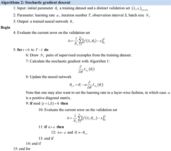
The training of a neural network consists in determining and empirically calculating the value of each of its parameters. The principle is as follows: the network processes an image and at the output it makes a prediction, that is to say that it tells which class it thinks this image belongs to. Knowing that we already know the class of each training image, we can check if this result is correct. Depending on the veracity of this result, we update all the network parameters, according to an algorithm called backpropagation of the error gradient. The aim of the gradient algorithm is to converge iteratively towards an optimal configuration of the synaptic weights (parameters). This state can be a local minimum of the function to be optimized and ideally a global minimum of this function, called the cost function. The weights in the neural network are first initialized with random values. We then consider a set of data that will be used for learning. Each sample has its target values which are those which the neural network must ultimately predict when presented with the same sample. The “Stochastic gradient descent” algorithm provides our trained neural network. It uses the “Backpropagation” algorithm to calculate the stochastic gradient. The two algorithms are presented below.

References

- 1. CNRA (2006) Bulletin d’information et de liaison du Centre National de Recherche Agronomique N° 18 Août 2006.
- 2. Deng, L., Yu, D., et al. (2014) Deep Learning: Methods and Applications, Foundations and Trends R in Signal Processing, 7, 197-387. https://doi.org/10.1561/2000000039
- 3. Premaladha, J. and Ravichandran, K. (2016) Novel Approaches for Diagnosing Melanoma Skin Lesions through Supervised and Deep Learning Algorithms. Journal of Medical Systems, 40, 96. https://doi.org/10.1007/s10916-016-0460-2
- 4. Kharazmi, P., Zheng, J., Lui, H., Wang, Z.J. and Lee, T.K. (2018) A Computer-Aided Decision Support System for Detection and Localization of Cutaneous Vasculature in Dermoscopy Images via Deep Feature Learning. Journal of Medical Systems, 42, 33. https://doi.org/10.1007/s10916-017-0885-2
- 5. Wang, S.-H., Phillips, P., Sui, Y., Liu, B., Yang, M. and Cheng, H. (2018) Classification of Alzheimers Disease Based on Eight-Layer Convolutional Neural Network with Leaky Rectified Linear Unit and Max Pooling. Journal of Medical Systems, 42, 85. https://doi.org/10.1007/s10916-017-0885-2
- 6. LeCun, Y., Bottou, L., Bengio, Y. and Haffner, P. (1998) Gradient-Based Learning Applied to Document Recognition, Proceedings of the IEEE, 86, 2278-2324. https://doi.org/10.1109/5.726791
- 7. Delalleau, O. (2012) Apprentissage machine efficace: Théorie et pratique. Thèse de doctorat, Université de Montreal, Montreal.
- 8. Labelle, J. (1981) Theorie des graphes. Modulo, Montréal.
- 9. Zeiler, M. and Fergus, R. (2013) Visualizing and Understanding Convolutional Networks. arXiv:1311.2901
- 10. LeCun, Y. (1988) A Theoretical Framework for Back-Propagation. In: Touretzky, D., Hinton, G. and Sejnowski, T., Eds., Proceedings of the 1988 Connectionist Models Summer School, CMU, Pittsburg, PA.
- 11. Copeland, M. (2006) What’s the Difference between Artificial Intelligence, Machine Learning, and Deep Learning? The Canadian Press.
- 12. Lerman, L. (2011) Les systemes de detection d’intrusion bases sur du machine learning.