Applied Mathematics
Vol.08 No.09(2017), Article ID:78918,18 pages
10.4236/am.2017.89093

A Study of Weighted Polynomial Approximations with Several Variables (II)

Ryozi Sakai

Department of Mathematics, Meijo University, Tenpaku-ku, Nagoya, Japan

Copyright © 2017 by author and Scientific Research Publishing Inc.

This work is licensed under the Creative Commons Attribution International License (CC BY 4.0).

http://creativecommons.org/licenses/by/4.0/

Received: August 13, 2017; Accepted: September 3, 2017; Published: September 6, 2017

ABSTRACT

In this paper we investigate weighted polynomial approximations with several variables. Our study relates to the approximation for W f L p ( s ) by weighted polynomial. Then we will give some results relating to the Lagrange interpolation, the best approximation, the Markov-Bernstein inequality and the Nikolskii-type inequality.

Keywords:

Weighted Polynomial Approximations, the Lagrange Interpolation, the Best of Approximation, Inequalities

1. Introduction

Let s : = × × × ( s times, s 1 integer) be the direct product space, and let W ( x 1 , x 2 , , x s ) : = w 1 ( x 1 ) w 2 ( x 2 ) w s ( x s ) , where w i ( x i ) 0 be even weight functions. We suppose that for every nonnegative integer n,

0 x n w i ( x ) d x < , n = 0 , 1 , 2 , , i = 1 , 2 , , s .

In this paper we will study to approximate the real-valued weighted function ( W f ) ( x 1 , x 2 , , x s ) by weighted polynomials ( W P ) ( x 1 , x 2 , , x s ) , where P ( x 1 , x 2 , , x s ) P n , n , , n ( s ) . Here, P n , n , , n ( s ) ( = : P n ; s ( s ) ) means a class of all polynomials with at most n-degree for each variable x i , i = 1 , 2 , , s . We need to define the norms. Let 0 < p , and let f : s be measurable. Then we define

W f L p ( s ) : = { [ | ( W f ) ( x 1 , , x s ) | p d x 1 d x s ] 1 / p , if 0 < p < ; sup ( x 1 , , x s ) s | ( W f ) ( x 1 , , x s ) | , if p = .

We assume that for 0 < p the integral is independent of the order of integration with respect to each x i , i = 1 , 2 , , s . When W f L p ( s ) < , we write W f L p ( s ) . If p = , we require that f is continuous and l i m | X | W ( X ) f ( X ) = 0 , where | X | = | ( x 1 , , x s ) | = max | x i | ; i = 1 , 2 , , s . Then we write W f C 0 ( s ) .

Our purpose in this paper is to approximate the weighted function W f L p ( s ) by weighted polynomials W P ; P P n ; s ( s ) . In Section 2, we give a class of the weights which are treated in this paper. In Section 3, we state our main theorems. First, we consider the Lagrange interpolation polynomials. Next, we give the necessary and sufficient conditions for the best approximation. In Sections 4 and 5, we will prove theorems.

2. Class of Weight Functions and Preliminaries

Throughout the paper C , C 1 , C 2 , denote positive constants independent of n , x , t or polynomials P ( x ) . The same symbol does not necessarily denote the same constant in different occurrences. Let f ( x ) ~ g ( x ) mean that there exists a constant C > 0 such that C 1 f ( x ) g ( x ) C f ( x ) holds for all x I , where I is a subset.

We say that f : [ 0, ) is quasi-increasing if there exists C > 0 such that f ( x ) C f ( y ) for 0 < x < y . Hereafter we consider following weights.

Definition 2.1. Let Q : [ 0, ) be a continuous and even function, and satisfy the following properties:

(a) Q ( x ) is continuous in , with Q ( 0 ) = 0 .

(b) Q ( x ) exists and is positive in \ { 0 } .

(c) lim x Q ( x ) = .

(d) The function

T ( x ) : = x Q ( x ) Q ( x ) , x 0

is quasi-increasing in ( 0, ) , with

T ( x ) Λ > 1 , x \ { 0 } .

(e) There exists C 1 > 0 such that

Q ( x ) | Q ( x ) | C 1 | Q ( x ) | Q ( x ) , a . e . x .

Then we write w = e x p ( Q ) F ( C 2 ) .

Moreover, if there also exists a compact subinterval J ( 0 ) of , and C 2 > 0 such that

Q ( x ) | Q ( x ) | C 2 | Q ( x ) | Q ( x ) , a . e . x \ J ,

then we write w = exp ( Q ) F ( C 2 + ) . If T ( x ) is bounded, then the weight w = e x p ( Q ) F ( C 2 + ) is called a Freud-type weight, and if T ( x ) is unbounded, then w is called an Erdös-type weight.

Let w ( x ) = e x p ( Q ( x ) ) F ( C 2 + ) , 0 < λ < ( m + 2 ) / ( m + 1 ) and m 1 be an integer. Then we write w F λ ( C m + 2 + ) if Q is C m + 2 -class and there exist C 1 and K 1 such that for all | x | K ,

| Q ( x ) | Q ( x ) λ C (2.1)

and

| Q ( x ) Q ( x ) | ~ | Q ( k + 1 ) ( x ) Q ( k ) ( x ) |

for every k = 2 , , m and also

| Q ( m + 2 ) ( x ) Q ( m + 1 ) ( x ) | | Q ( m + 1 ) ( x ) Q ( m ) ( x ) | .

Specific examples are shown in the following:

Example 2.2 (cf. [1] [2] ). (1) If an exponential Q ( x ) satisfies

1 < Λ 1 ( x Q ( x ) ) Q ( x ) Λ 2 ,

where Λ i , i = 1 , 2 are constants, then we call w = exp ( Q ( x ) ) the Freud weight. The class F ( C 2 + ) contains the Freud weights.

(2) For α > 1 , l 1 we define

Q ( x ) = Q l ; α ( x ) = exp l ( | x | α ) exp l ( 0 ) ,

where exp l ( x ) = exp ( exp ( exp exp x ) ) ( l times ) . Moreover, we define

Q l ; α , m ( x ) = | x | m { exp l ( | x | α ) α * exp l ( 0 ) } , α + m > 1 , m 0 , α 0 ,

where α * = 0 if α = 0 , and otherwise α * = 1 . We note that Q l ; 0, m gives a Freud-type weight, that is, T ( x ) is bounded..

(3) We define

Q α ( x ) = ( 1 + | x | ) | x | α 1 , α > 1.

(4) Let w = e x p ( Q ) F ( C 2 + ) , and let us define

μ + : = lim sup x Q ( x ) Q ( x ) / Q ( x ) Q ( x ) , μ : = lim inf x Q ( x ) Q ( x ) / Q ( x ) Q ( x ) .

If μ + = μ , then we say that the weight w is regular. All weights in examples (1), (2) and (3) are regular.

(5) More generally we can give the examples of weights w F λ ( C m + 2 + ) . If the weight w is regular and if Q C m + 2 ( \ { 0 } ) satisfies definition (2.1), then for the regular weights we have w F λ ( C m + 2 + ) (see [3] , Corollary 5.5 (5.8)).

Proposition 2.3 ( [3] , Theorem 4.2 and (4.11)). Let m be a positive integer, 0 < λ < ( m + 2 ) / ( m + 1 ) and let w = e x p ( Q ) F λ ( C m + 2 + ) . Then for μ , ν , α , β , we can construct a new weight w μ , ν , α , β F λ ( C m + 1 + ) F ( C 2 + ) such that

T w ( x ) μ ( 1 + x 2 ) ν ( 1 + Q ( x ) ) α ( 1 + | Q ( x ) | ) β w ( x ) ~ w μ , ν , α , β ( x ) on ,

and for some C 1 ,

a n / C ( w μ , ν , α , β ) a n ( w ) a C n ( w μ , ν , α , β ) and T w μ , ν , α , β ( x ) ~ T w ( x ) = T ( x ) ,

where a n ( w μ , ν , α , β ) and a n ( w ) are MRS-numbers for the weight w μ , ν , α , β or w , respectively, and T w μ , ν , α , β , T w are correspond for w μ , ν , α , β or w, respectively.

Let { p n } be orthonormal polynomials with respect to a weight w, that is, p n is the polynomial of degree n such that

p n ( x ) p m ( x ) w 2 ( x ) d x = δ m n ( theKroneckerdelta ) .

For 1 p , we denote by L p ( ) the usual L p space on (here for p = , if w f L ( ) then we require f to be continuous, and f w to have limit 0 at ± ). Let w F ( C 2 + ) . We need the Mhaskar-Rakhmanov-Saff numbers (MRS numbers) a x ;

x = 2 π 0 1 a x u Q ( a x u ) ( 1 u 2 ) 1 / 2 d u , x > 0.

we see easily

lim x a x = and lim x + 0 a x = 0

and

lim x a x x = 0 and lim x + 0 a x x = .

For w f L p ( ) ( 1 p ) the degree of weighted polynomial approximation is defined by

E n , p ( w ; f ) : = i n f P P n w ( f P ) L p ( ) .

3. Main Results

Let w i F ( C 2 + ) , i = 1,2, , s , and let W ( X ) = i = 1 s w i ( x i ) , where X = ( x 1 , x 2 , , x s ) s . Then we have the following theorem.

Theorem 3.1 ( [4] , Theorem 3.3). We suppose w j = exp ( Q j ) F λ ( C 3 + ) ( 0 < λ < 3 / 2 ) , j = 1 , 2 , , s and let

T j ( a n ( j ) ) c ( n a n ( j ) ) 2 / 3 , j = 1 , 2 , , s .

If i = 1 s { T i 1 / 4 w i } f C 0 ( s ) , then there exist P n P n ; s ( s ) , n = 1 , 2 , 3 , such that we have

W ( f P n ) L ( s ) 0 as n .

First, we consider the Lagrange interpolation operators. We construct the orthonormal polynomials p n , i with respect to the weight w i for each i = 1 , 2 , , s . Let x n , n , i < x n 1 , n , i < < x 1 , n , i , i = 1 , 2 , , s are zeros of the orthonormal polynomial p n , i , that is, p n , i ( x k i , n , i ) = 0 , k i = 1 , 2 , , n and put S n = { ( x k 1 , n , 1 , , x k s , n , s ) ; 1 k i n , i = 1 , 2 , , s } . Then for W f C 0 ( ) we define the Lagrange interpolation polynomial on S n as

L n ( f ; x 1 , , x s ) = k s = 1 n k 1 = 1 n f ( x k 1 , n , 1 , , x k s , n , s ) i = 1 s l k i , n , i ( x i ) , (3.1)

where

l k i , n , i ( x i ) = p n , i ( x i ) ( x i x k i , n , i ) p n , i ( x k i , n , i ) . (3.2)

In the rest of this paper, if w i , i = 1 , 2 , , s are the Freud-type weights then we suppose a n ( i ) = o ( 1 ) n 2 / 3 .

Theorem 3.2. Let w i F ( C 2 + ) , i = 1,2, , s , and let f : s be continuous. If

i = 1 s { ( 1 + x i 2 ) β / 2 w i ( x i ) } | f ( x 1 , , x s ) | C 0 ( s ) (3.3)

holds, then there exists n 0 > 0 such that for n n 0

| k s = 1 n k 1 = 1 n i = 1 s λ k i , n , i f ( x k 1 , n , 1 , , x k s , n , s ) | C i = 1 s { ( 1 + x i 2 ) β w i 2 ( x i ) } f ( x 1 , , x s ) L ( s ) , (3.4)

where for each i = 1 , 2 , , s , x k i , n , i ( k i = 1 , 2 , , n ) are zeros of p n , i ( x i ) . In particular,

lim n k s = 1 n k 1 = 1 n i = 1 s λ k i , n , i f ( x k 1 , n , 1 , , x k s , n , s ) = i = 1 s w i 2 ( x i ) f ( x 1 , , x s ) d x 1 d x s . (3.5)

Theorem 3.3. Let w i F λ ( C 3 + ) ( 0 < λ < 3 / 2 ) , i = 1 , 2 , 3 , , s . Let β > 1 / 2 , and let f : s satisfy (3.3), then we have for n = 1 , 2 , ,

i = 1 s w i L n ( f ) L ( s ) C i = 1 s { ( 1 + x i 2 ) ( β / 2 ) w i ( x i ) } f ( x 1 , , x s ) L ( s ) , (3.6)

where for each i = 1 , 2 , , s , x k i , n , i , k i = 1 , 2 , , n are zeros of p n , i ( x i ) . In

particular, if i = 1 s { ( 1 + x i 2 ) ( β / 2 ) T i 1 / 4 ( x i ) w i ( x i ) } f ( x 1 , , x s ) C 0 ( s ) , then we

have

lim n i = 1 s w i ( f L n ( f ) ) L 2 ( s ) = 0.

For p 2 we also obtain the similar results. We need a function as follows:

Ψ ( x ) : = 1 ( 1 + Q ( x ) ) 2 / 3 T ( x ) . (3.7)

Theorem 3.4. Let w i F λ ( C 3 + ) , 0 < λ < 3 / 2 ( i = 1 , 2 , , s ) . Let 1 < p 2 and β > 1 / p , and let Ψ ( x ) be defined by (3.7) for each w i , i = 1 , 2 , , s . If f : is continuous, and satisfies

| i = 1 s { ( 1 + x i 2 ) β / 2 T i 1 / 2 ( x i ) Ψ i 1 / 4 ( x i ) } W ( X ) f ( X ) | < , X s , i = 1 , 2 , , s , (3.8)

then we have

W L n ( f ) L p ( s ) C i = 1 s { ( 1 + x i 2 ) β / 2 T i 1 / 2 ( x i ) Ψ i 1 / 4 ( x i ) } W f L ( s ) , n = 1 , 2 , . (3.9)

Especially, if f satisfies

| i = 1 s { ( 1 + x i 2 ) β / 2 T i 3 / 4 ( x i ) Ψ i 1 / 4 ( x i ) } W ( X ) f ( X ) | C o ( s ) , (3.10)

then we have

lim n W ( f L n ( f ) ) L p ( s ) = 0. (3.11)

For 2 < p we have the following:

Theorem 3.5. Let w i F λ ( C 3 + ) , 0 < λ < 3 / 2 ( i = 1 , 2 , , s ) , and let satisfy T i ( a n ( i ) ) C n 1 / 2 . Let 2 < p and β > 1 / p . Furthermore we assume

Q i ( a n ( i ) 4 ) C ( l o g ( Q i ( a n ( i ) ) ) ) 4 , i = 1,2, , s . (3.12)

If f : s is continuous, and satisfies

| i = 1 s { ( 1 + x i 2 ) β / 2 T i 1 / 2 ( x i ) Ψ i 1 ( x i ) } W ( X ) f ( X ) | < , X s , (3.13)

then we have

{ i = 1 s Ψ i 3 / 4 ( x i ) } W L n ( f ) L p ( s ) C i = 1 s { ( 1 + x i 2 ) β / 2 T i 1 / 2 ( x i ) Ψ i 1 / 4 ( x i ) } W f L ( s ) .

Especially, by (3.13) we have

lim n { i = 1 s Ψ i 3 / 4 ( x i ) } W ( f L n ( f ) ) L p ( s ) = 0.

Remark 3.6. (1) We note that (3.13) means

( i = 1 s T i 1 / 4 ) W * f C 0 ( s ) ,

where i = 1 s { ( 1 + x i 2 ) β / 2 T i 1 / 2 ( x i ) Ψ i 1 / 4 ( x i ) } W ~ W * F ( C 2 + ) (see Theorem 2.3).

(2) All examples in Example 2.2 hold (3.12).

(3) To prove Theorem 3.5 we use Proposition 4.5. Then Assumption (3.12) plays an important role.

Next, we characterize the best approximation polynomial (cf. [5] ).

Theorem 3.7. Let 0 < p . There is a best approximation polynomial P f P n ; s such that

E p , n ; s ( W , f ) : = i n f P P n ; s W ( f P ) L p ( s ) = W ( f P n ; f ) L p ( s ) .

Theorem 3.8 (Kolmogorov-type theorem). P P n ; s is a best of approximation for a continuous function f with l i m | ( x 1 , , x s ) | W ( x 1 , , x s ) f ( x 1 , , x s ) = 0 , if and only if for each polynomial Q P n ; s ,

m a x ( x 1 , , x s ) A [ W ( x 1 , , x s ) ( f ( x 1 , , x s ) P ( x 1 , , x s ) ) ] Q ( x 1 , , x s ) 0, (3.14)

where A denotes the set (which depends on f and P ) of all points ( x 1 , , x s ) A for which

| W ( x 1 , , x s ) ( f ( x 1 , , x s ) P ( x 1 , , x s ) ) | = W ( f P ) L ( s ) .

Theorem 3.9. Let W = i = 1 s w i , w i F ( C 2 + ) , i = 1 , , s and 1 p < . Let ϕ K , where K = ( k 1 , , k s ) ( 0 k j n ) ( j = 1 , , s ) be a linearly independent system satisfying W ϕ K L p ( s ) , and we consider polynomials

Q ( X ) = k s = 1 n k 1 = 1 n c ( k 1 , , k s ) ϕ ( k 1 , , k s ) ( X ) . (3.15)

Let W f L p ( s ) . The polynomial

P ( X ) = k s = 1 n k 1 = 1 n c ( k 1 , , k s ) [ 0 ] ϕ ( k 1 , , k s ) ( X ) (3.16)

is a polynomial of the best approximation for f if and only if for every polynomial (3.15) the following equality (3.17) holds.

s Q ( X ) | f ( X ) P ( X ) | p 1 [ sign ( f ( X ) P ( X ) ) ] W p ( X ) D X : = Q ( x 1 , , x s ) | f ( x 1 , , x s ) P ( x 1 , , x s ) | p 1 × [ sign ( f ( x 1 , , x s ) P ( x 1 , , x s ) ) ] W p ( x 1 , , x s ) d x 1 d x s = 0 (3.17)

holds. If p = 1 , we also assume that f ( X ) P ( X ) vanish only on a set of measure zero.

4. Proofs of Theorems 3.2, 3.3, 3.4 and 3.5

Lemma 4.1. Let x n , n , i < x n 1 , n , i < < x 1 , n , i be zeros of the orthonormal polynomial p n , i , and let

P n 1 ( x 1 , x 2 , , x s ) = 0 j i n 1 , i = 1 , 2 , , s a j 1 , , j s x 1 j 1 x s j s ,

where a j 1 , , j s are coefficients. If for every ( x k 1 , n ,1 , , x k s , n , s ) ,

P n 1 ( x k 1 , n , 1 , , x k s , n , s ) = 0 , 1 k i n , i = 1 , , s , (4.1)

then we have P n 1 = 0 . Therefore, for P n 1 ( x 1 , x 2 , , x s ) P n 1 ( s ) we have

P n 1 = L n ( P n 1 ) . (4.2)

Proof. Now we fix any ( x k 2 , n , 2 , , x k s , n , s ) s 1 , and then we consider the polynomial Q n 1 ( x 1 ) in P n 1 ( ) such that

Q n 1 ( x 1 ) = j 1 = 0 n 1 ( 0 j i n 1 , i = 2 , 3 , , s a j 1 , , j s x k 2 , n , 2 j 2 x k s , n , s j s ) x 1 j 1 .

Since

Q n 1 ( x k 1 , n , 1 ) = 0 , k 1 = 1 , 2 , , n

(see (4.1)), all coefficients of Q n 1 ( x 1 ) equal to zero, that is,

0 j i n 1 , i = 2 , 3 , , s a j 1 , , j s x k 2 , n , 2 j 2 x k s , n , s j s = 0 , for each j 1 = 0 , 1 , , n 1. (4.3)

Next, we fix any

j 1 ( 0 j 1 n 1 ) and ( x k 3 , n ,3 , , x k s , n , s ) s 2 ,

and we consider R n 1 P n 1 ( ) such that

R n 1 ( x 2 ) = j 2 = 0 n 1 ( 0 j i n 1 , i = 3 , 4 , , s a j 1 , , j s x k 3 , n , 3 j 3 x k s , n , s j s ) x 2 j 2 .

Then by (4.3), we see

R n 1 ( x k 2 , n , 2 ) = 0 , k 2 = 1 , 2 , , n .

Hence,

0 j i n 1 , i = 3 , 4 , , s a j 1 , , j s x 3 , k 3 j 3 x s , k s j s = 0 , for each j 1 , j 2 = 0 , 1 , , n 1.

If we continue this method inductively, then we have

j s = 0 n 1 a j 1 , , j s x k s , n , s j s = 0 , for each j 1 , j 2 , , j s 1 = 0 , 1 , , n 1. (4.4)

We put H n 1 P n 1 ( ) as

H n 1 ( x s ) = j s = 0 n 1 a j 1 , , j s x s j s ,

then from (4.4) we have H n 1 ( x k s , n , s ) = 0 , k s = 1 , 2 , , n . Therefore, we conclude

a j 1 , , j s = 0 , j i = 0 , 1 , , n 1 ( i = 1 , 2 , , s ) ,

that is, P n 1 = 0 . #

In the rest of this paper, we use the following notations:

W = i = 1 s w i , X = ( x 1 , , x s ) , X ( u ) = ( u 1 , , u s )

D ( X ) = d x 1 d x s , D ( X ( u ) ) = d u 1 d u s .

We also use

P n ; s ( s ) : = P n , , n ( s ) : = { P n | P n ( x 1 , , x s ) arepolynomialswithdegree n for each x i , i = 1 , , s } .

Proposition 4.2 (cf. [6] , Theorem 1.2.2). Let w i F ( C 2 + ) , i = 1,2, , s , and let n 1 be an integer. Then for all P P 2 n 1 ; s ( s ) , we have

s P ( X ( u ) ) W 2 ( X ( u ) ) D ( X ( u ) ) = k s = 1 n k 1 = 1 n λ k 1 , n ,1 λ k s , n , s P ( x k 1 , n ,1 , , x k s , n , s ) , (4.5)

where

λ k i , n , i = l k i , n , i w i 2 ( x i ) d x i , i = 1 , 2 , , s . (4.6)

Proof. (see [6] , pp.12-13). Let P P n 1 ; s ( s ) . From (3.1) and (4.2) we see

P ( X ) = L n ( P ; X ) = k s = 1 n k 1 = 1 n l k 1 , n , 1 ( x 1 ) l k s , n , s ( x s ) P ( x k 1 , n , 1 , , x k s , n , s ) .

Hence we have

s P ( X ( u ) ) W 2 ( X ( u ) ) D ( X ( u ) ) = k s = 1 n k 1 = 1 n λ k 1 , n , 1 λ k s , n , s P ( x k 1 , n , 1 , , x k s , n , s ) ,

that is, (4.5) holds. Now, we see that (4.5) holds for any P P 2 n 1 ; s ( s ) . In fact, for P P 2 n 1 ; s ( s ) we set

P ( x 1 , , x s ) = Q ( x 1 , , x s ) i = 1 s p n , i ( x i ) + R ( x 1 , , x s ) , Q , R P n 1 , , n 1 ( s ) .

Then

s P ( X ( u ) ) W ( X ( u ) ) D ( X ( u ) ) = s Q ( X ( u ) ) i = 1 s p n , j i ( u j i ) W ( X ( u ) ) D ( X ( u ) ) + s R ( X ( u ) ) W ( X ( u ) ) D ( X ( u ) ) = s R ( X ( u ) ) W ( X ( u ) ) D ( X ( u ) ) = k s = 1 n k 1 = 1 n λ k 1 , n , 1 λ k s , n , s R ( x k 1 , n , 1 , , x k s , n , s ) = k s = 1 n k 1 = 1 n λ k 1 , n , 1 λ k s , n , s ( Q ( x k 1 , n , 1 , , x k s , n , s ) i = 1 s p n , i ( x k i , n , i ) + R ( x k 1 , n , 1 , , x k s , n , s ) ) = k s = 1 n k 1 = 1 n λ k 1 , n , 1 λ k s , n , s P ( x k 1 , n , 1 , , x k s , n , s ) ,

that is, (4.5) holds for any P P 2 n 1 ; s ( s ) . #

Lemma 4.3 ( [7] , Theorem 2.1). Let w = exp ( Q ) F ( C 2 + ) , b . If w is a Freud-type weight, then we assume a n = o ( 1 ) n 2 / 3 . Then there exist constants C 1 , C 2 > 0 such that for every integer n 1 ,

C 1 a n a n ( 1 + x 2 ) b d x j = 1 n λ k , n w 2 ( x k , n ) ( 1 + x k , n 2 ) b C 2 a n a n ( 1 + x 2 ) b d x .

Proof of Theorem 3.2.
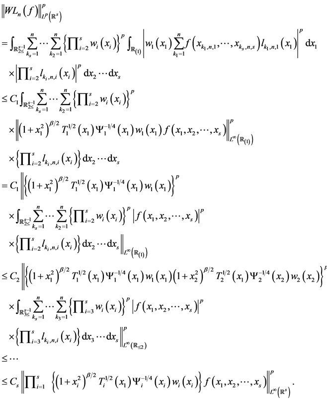
k s = 1 n k 1 = 1 n i = 1 s λ k i , n , i | f ( x k 1 , n , 1 , , x k s , n , s ) | i = 1 s { ( 1 + x i 2 ) β w i 2 ( x i ) } f ( x 1 , , x s ) L ( s ) s = 1 n i = 1 n i = 1 s { λ k i , n , i w i 2 ( x k i , n , i ) ( 1 + x k i , n , i 2 ) β } i = 1 s { ( 1 + x i 2 ) β w i 2 ( x i ) } f ( x 1 , , x s ) L ( s ) a n [ s ] a n [ s ] a n [ 1 ] a n [ 1 ] i = 1 s ( 1 + x i 2 ) β d x 1 d x s

by Lemma 4.3

C i = 1 s { ( 1 + x i 2 ) β w i 2 ( x i ) } f ( x 1 , , x s ) L ( s ) .

Therefore we have (3.4). To prove (3.5) we use (3.4) and Proposition 4.2. For P P n ; s ( s ) we see

| k s = 1 n k 1 = 1 n { i = 1 s λ k i , n , i } f ( x k 1 , n , 1 x k s , n , s ) f ( x 1 , , x s ) w 1 2 ( x 1 ) w s 2 ( x s ) d x 1 d x s | | k s = 1 n k 1 = 1 n { i = 1 s λ k i , n , i } ( f P ) ( x k 1 , n , 1 x k s , n , s ) | + | ( f P ) ( x 1 , , x s ) w 1 2 ( x 1 ) w s 2 ( x s ) d x 1 d x s | | k s = 1 n k 1 = 1 n { i = 1 s λ k i , n , i } ( f P ) ( x k 1 , n , 1 x k s , n , s ) | + | ( f P ) ( x 1 , , x s ) w 1 2 ( x 1 ) w s 2 ( x s ) d x 1 d x s | C i = 1 s { ( 1 + x i 2 ) β w i 2 ( x i ) } ( f P ) ( x 1 , , x s ) L ( s ) + i = 1 s { ( 1 + x i 2 ) β w i 2 ( x i ) } ( f P ) ( x 1 , , x s ) L ( s ) × i = 1 s ( 1 + x i 2 ) β d x 1 d x s C i = 1 s { ( 1 + x i 2 ) β w i 2 ( x i ) } ( f P ) ( x 1 , , x s ) L ( s ) .

Now, we can take P = P n as

l i m n i = 1 s { ( 1 + x i 2 ) β w i 2 ( x i ) } ( f P n ) ( x 1 , , x s ) L ( s ) = 0. (4.7)

In fact, when we put i = 1 s ( 1 + x i 2 ) β w i 2 ( x i ) ~ W β F ( C 2 + ) (see Proposition 2.3), from (3.3) we see

i = 1 s { T i 1 / 4 ( x i ) ( 1 + x i 2 ) β w i 2 } f C i = 1 s { ( 1 + x i 2 ) β w i ( x i ) } f C 0 ( s ) .

Hence from Theorem 3.1 with W β we have (4.7). Therefore we conclude (3.5). #

Proof of Theorem 3.3. By Proposition 4.2 with P = L n 2 ( f ) and Theorem 3.2 with (3.4),

i = 1 s w i L n ( f ) L 2 ( s ) = k s = 1 n k 1 = 1 n { i = 1 s λ k i , n , i } { L n ( f ; x k 1 , n , 1 x k s , n , s ) } 2 = k s = 1 n k 1 = 1 n { i = 1 s λ k i , n , i } { f ( x k 1 , n , 1 x k s , n , s ) } 2 C i = 1 s { ( 1 + x i 2 ) β w i 2 ( x i ) } { f ( x 1 , , x s ) } 2 L ( s ) = C i = 1 s { ( 1 + x i 2 ) ( β / 2 ) w i ( x i ) } f ( x 1 , , x s ) L ( s ) 2 ,

that is, we have (3.6). From Theorem 4.1 with

i = 1 s ( 1 + x i 2 ) β / 2 w i 2 ( x i ) ~ W β / 2 F ( C 2 + ) (note Proposition 2.3) and our assumption, there exists P n 1 P n 1 such that

l i m n i = 1 s { ( 1 + x i 2 ) ( β / 2 ) w i ( x i ) } ( f P n 1 ) ( x 1 , , x s ) L ( s ) 2 = 0.

Then

W ( f L n ( f ) ) L 2 ( s ) W ( f P n 1 ) L 2 ( s ) + W L n ( f P ) L 2 ( s ) i = 1 s { ( 1 + x i 2 ) ( β / 2 ) w i ( x i ) } ( f P n 1 ) ( x 1 , , x s ) L ( s ) 2 i = 1 s ( 1 + x i 2 ) ( β / 2 ) L 2 ( s ) + i = 1 s { ( 1 + x i 2 ) ( β / 2 ) w i ( x i ) } ( f P n 1 ) ( x 1 , , x s ) L ( s ) 2 C i = 1 s { ( 1 + x i 2 ) ( β / 2 ) w i ( x i ) } ( f P n 1 ) ( x 1 , , x s ) L ( s ) 2 0 as n . #

We know the following propositions with respect to one variable.

Proposition 4.4 ( [8] , Theorem 2.7). Let w F λ ( C 3 + ) , 0 < λ < 3 / 2 . Let 1 < p 2 and β > 1 / p . If f : s is continuous, and satisfies

| ( 1 + x 2 ) β / 2 T 1 / 2 ( x ) Ψ 1 / 4 ( x ) w ( x ) f ( x ) | < , x ,

then we have

w L n ( f ) L p ( ) C ( 1 + x 2 ) β / 2 T 1 / 2 ( x ) Ψ 1 / 4 ( x ) w f L ( ) , n = 1,2, . (4.8)

Especially, if

| ( 1 + x 2 ) β / 2 T 1 / 2 ( x ) Ψ 1 / 4 ( x ) w ( x ) f ( x ) | C 0 ( ) ,

then we have

lim n w ( f L n ( f ) ) L p ( ) = 0.

Proposition 4.5 ( [8] , Theorem 2.8). Let w F λ ( C 3 + ) , 0 < λ < 3 / 2 , and let satisfy T i ( a n ( i ) ) C n 1 / 2 . Let 2 < p and β > 1 / p . Furthermore we assume

Q ( a n 4 ) C ( l o g ( Q ( a n ) ) ) 4 .

If f : satisfies

| ( 1 + x 2 ) β / 2 T 1 / 2 ( x ) Ψ 1 / 4 ( x ) w ( x ) f ( x ) | C , x ,

then we have

Ψ 3 / 4 ( x ) w L n ( f ) L p ( ) C ( 1 + x 2 ) β / 2 T 1 / 2 ( x ) Ψ 1 / 4 ( x ) w f L ( ) , n = 1 , 2 , . (4.9)

Especially, if

| ( 1 + x 2 ) β / 2 T 1 / 2 ( x ) Ψ 1 / 4 ( x ) w ( x ) f ( x ) | C 0 ( ) ,

we have

lim n w ( f L n ( f ) ) L p ( ) = 0.

Proof of Theorem 3.4. We use Proposition 4.4 (4.8).

Hence we have (3.9).

Next we show (3.10). There exists P n P n ; s ( s ) such that

i = 1 s { ( 1 + x i 2 ) β / 2 T i 1 / 2 ( x i ) Ψ i 1 / 4 ( x i ) } W ( f P n ) L ( s ) C E , n ; s ( i = 1 s { ( 1 + x i 2 ) β / 2 T i 1 / 2 ( x i ) Ψ i 1 / 4 ( x i ) } W , f )

i = 1 s { ( 1 + x i 2 ) β / 2 T i 1 / 2 ( x i ) Ψ i 1 / 4 ( x i ) } W ( f P n ) L ( s ) C E , n ; s ( i = 1 s { ( 1 + x i 2 ) β / 2 T i 1 / 2 ( x i ) Ψ i 1 / 4 ( x i ) } W , f ) ,

where P n P n ; s . Then

W ( f L n ( f ) ) L p ( s ) W ( f P n ) L p ( s ) + W L n ( f P n ) L p ( s ) W ( f P n ) L p ( s ) + C i = 1 s { ( 1 + x i 2 ) β / 2 T i 1 / 2 ( x i ) Ψ i 1 / 4 ( x i ) } W ( f P n ) L ( s ) i = 1 s { ( 1 + x i 2 ) β / 2 T i 1 / 2 ( x i ) Ψ i 1 / 4 ( x i ) } W ( f P n ) L ( s ) × i = 1 s { ( 1 + x i 2 ) β / 2 T i 1 / 2 ( x i ) Ψ i 1 / 4 ( x i ) } L p ( s ) + C i = 1 s { ( 1 + x i 2 ) β / 2 T i 1 / 2 ( x i ) Ψ i 1 / 4 ( x i ) } W ( f P n ) L ( s ) C E , n ; s ( i = 1 s { ( 1 + x i 2 ) β / 2 T i 1 / 2 ( x i ) Ψ i 1 / 4 ( x i ) } W , f ) 0 as n 0.

The last convergence follows from (3.9) and Theorem 3.1 with

i = 1 s { ( 1 + x i 2 ) β / 2 T i 1 / 2 ( x i ) Ψ i 1 / 4 ( x i ) } ~ W * F ( C 2 + ) (note Proposition 2.3). Consequently, we have (3.11). #

Proof of Theorem 3.5. As the proof of Theorem 3.4 we can show Theorem 3.5 by Proposition 4.5 (4.9). Then we also note Remark 3.6 (1) and (3). #

5. Proofs of Theorems 3.7, 3.8 and 3.9

In this section, we characterize the best approximation polynomial (cf. [5] ).

Proof of Theorem 3.7. We consider the polynomial class

T = { P ( x 1 , , x s ) = k i = 0 , 1 i s n a k 1 , , k s x 1 k 1 x s k s ; ( f P ) W L p ( s ) f W L p ( s ) } .

Since

( f 0 ) W L p ( s ) = f W L p ( s ) ,

the set T is not empty. Now we select the sequence

{ P m , n ( x 1 , , x s ) = k i = 0 , 1 i s n a k 1 , , k s ; m x 1 k 1 x s k s } m = 0 such that

inf a k 1 , , k s ; m ( f P m , n ) W L p ( s ) = E p , n ; s ( W ; f ) .

Here we see that | a m | : = max k j = 0 , 1 , , n ; 1 j s | a k 1 , , k s ; m | is bounded. In fact, if it is unbounded, then for

Q m , n ( x 1 , , x s ) = P m , n ( x 1 , , x s ) / a m = k i = 0 , 1 i s n b k 1 , , k s ; m x 1 k 1 x s k s ,

we see | b k 1 , , k s ; m | 1 . Then we can take a subsequence { m l } l = 1 and a fixed term

x 1 k 1 ; 0 x s k s ; 0 such that

Q m l , n ( x 1 , , x s ) = x 1 k 1 , 0 x s k s , 0 + k i = 0 , k i k i , 0 , 1 i s n b k 1 , , k s ; m l x 1 k 1 x s k s .

We can suppose b k 1 , , k s ; m l b k 1 , , k s as l (if we need it, then we consider a subsequence). Now, we see that there exists M > 0 such that P m l W L ( s ) < M , so we have

Q m l , n W L ( s ) 0 ,

that is,

Q n ( x 1 , , x s ) : = x 1 k 1 ; 0 x s k s ; 0 + k i = 0 , k i k i , 0 , 1 i s n b k 1 , , k s x 1 k 1 x s k s = 0.

This is impossible because the { x 1 k 1 x s k s } are linear independent. Hence | a m | : = max k j = 0 , 1 , , n ; 1 j s | a k 1 , , k s ; m | is bounded. Now we repeat the method as above. If we select the sequence a k 1 , , k s ; m a k 1 , , k s as l (if we need it, then we consider a subsequence), then we have

( f k i = 0 , 1 i s n a k 1 , , k s x 1 k 1 x s k s ) W L p ( ) = E p , n ; s ( W ; f ) .

Then we put P n ; f : = k i = 0 , 1 i s n a k 1 , , k s x 1 k 1 x s k s . #

Proof of Theorem 3.8. Let

W ( f P n ; f ) L ( s ) = E n ; s ( W , f ) ,

where P n ; f P n ; s ( s ) . We see that the theorem is trivial if E n ; s ( W , f ) = 0 . So we may assume E n ; s ( W , f ) > 0 . If (3.14) is not true, there exists a polynomial Q P n ; s such that

m a x ( x 1 , , x s ) A [ W ( x 1 , , x s ) ( f ( x 1 , , x s ) P n ; f ( x 1 , , x s ) ) ] Q ( x 1 , , x s ) = 2 ε

for some ε > 0 . By the continuity of the function, there exists an open subset G ; A G , such that

W ( x 1 , , x s ) [ f ( x 1 , , x s ) P n ; f ( x 1 , , x s ) ] Q ( x 1 , , x s ) < ε , ( x 1 , , x s ) G .

For λ > 0 small enough we put R = P n ; f λ Q , and let

M = s u p ( x 1 , , x s ) s W ( x 1 , , x s ) | Q ( x 1 , , x s ) | .

First, for ( x 1 , , x s ) G we see

| W ( x 1 , , x s ) ( f ( x 1 , , x s ) R ( x 1 , , x s ) ) | 2 = | W ( x 1 , , x s ) ( f ( x 1 , , x s ) P n ; f ( x 1 , , x s ) + λ Q ( x 1 , , x s ) ) | 2 = | W ( x 1 , , x s ) ( f ( x 1 , , x s ) P n ; f ( x 1 , , x s ) ) | 2 + 2 λ [ W ( x 1 , , x s ) ( f ( x 1 , , x s ) P n ; f ( x 1 , , x s ) ) ] Q ( x 1 , , x s ) + λ 2 W 2 ( x 1 , , x s ) | Q ( x 1 , , x s ) | 2 < E n ; s ( W , f ) 2 2 λ ε + λ 2 M 2 .

If we take λ < M 2 ε , then we obtain

| W ( x 1 , , x s ) ( f ( x 1 , , x s ) R ( x 1 , , x s ) ) | 2 < E n ; s ( W , f ) 2 2 λ ε + λ ε = E n ; s ( W , f ) 2 λ ε , ( x 1 , , x s ) G . (5.1)

Next, we assume ( x 1 , , x s ) G c (the complement of G ). For large enough K 1 , K 2 > 0 there exists δ 1 > 0 such that

W ( x 1 , , x s ) | f ( x 1 , , x s ) | < E n ; s ( W , f ) 2 δ 1 , | ( x 1 , , x s ) | K 1 ,

and

W ( x 1 , , x s ) | P n ; f ( x 1 , , x s ) | < E n ; s ( W , f ) 2 δ 1 , | ( x 1 , , x s ) | K 2 ,

that is,

| W ( x 1 , , x s ) ( f ( x 1 , , x s ) P n ; f ( x 1 , , x s ) ) | < E n ; s ( W , f ) 2 δ 1 , | ( x 1 , , x s ) | m a x { K 1 , K 2 } .

Then we also see that there exists δ 2 > 0 such that

| W ( x 1 , , x s ) ( f ( x 1 , , x s ) P n ; f ( x 1 , , x s ) ) | < E n ; s ( W , f ) δ 2 , ( x 1 , , x s ) G c , | ( x 1 , , x s ) | max { K 1 , K 2 } .

Let δ : = min { 2 δ 1 , δ 2 } > 0 , and let ( x 1 , , x s ) G c . Then, if we take λ > 0 so small that λ < ( 2 M ) 1 δ , we see

| W ( x 1 , , x s ) ( f ( x 1 , , x s ) R ( x 1 , , x s ) ) | | W ( x 1 , , x s ) ( f ( x 1 , , x s ) P n ; f ( x 1 , , x s ) ) | + λ W ( x 1 , , x s ) | Q ( x 1 , , x s ) | E n ; s ( W , f ) δ + δ 2 = E n ; s ( W , f ) δ 2 . (5.2)

From (5.1) and (5.2) we see that the condition (3.14) is necessary.

Next we will show that (3.14) is also sufficient. Let R P n ; s be arbitrary polynomial. Then there exists a point ( x 1,0 , , x s ,0 ) A such that for Q = P R ,

[ W ( x 1 , , x s ) ( f ( x 1,0 , , x s ,0 ) P ( x 1,0 , , x s ,0 ) ) ] Q ( x 1,0 , , x s ,0 ) 0.

Then we see

| W ( x 1,0 , , x s ,0 ) ( f ( x 1,0 , , x s ,0 ) R ( x 1,0 , , x s ,0 ) ) | 2 = | W ( x 1,0 , , x s ,0 ) ( f ( x 1,0 , , x s ,0 ) P ( x 1,0 , , x s ,0 ) ) | 2 + 2 [ W ( x 1,0 , , x s ,0 ) ( f ( x 1,0 , , x s ,0 ) P ( x 1,0 , , x s ,0 ) ) ] Q ( x 1,0 , , x s ,0 ) + | W ( x 1,0 , , x s ,0 ) Q ( x 1,0 , , x s ,0 ) | 2 | W ( x 1,0 , , x s ,0 ) ( f ( x 1,0 , , x s ,0 ) P ( x 1,0 , , x s ,0 ) ) | 2 = W ( f P ) L ( ) 2 .

This means that there is not R with W ( f R ) L ( ) < W ( f P ) L ( ) , that is, P is the best of approximation polynomial. #

Proof of 3.9. Let the condition (3.17) be satisfied. We see

s | { f ( X ) P ( X ) } W ( X ) | p D ( X ) = s { f ( X ) P ( X ) } | f ( X ) P ( X ) | p 1 sign { f ( X ) P ( X ) } W p ( X ) D ( X ) = s { f ( X ) Q ( X ) } | f ( X ) P ( X ) | p 1 sign { f ( X ) P ( X ) } W p ( X ) D ( X ) s | f ( X ) Q ( X ) | | f ( X ) P ( X ) | p 1 W p ( X ) D ( X ) [ s | { f ( X ) Q ( X ) } W ( X ) | p D ( X ) ] 1 p [ s | { f ( X ) P ( X ) } W | p D ( X ) ] 1 1 p ,

that is,

[ s | { f ( X ) P ( X ) } W ( X ) | p D ( X ) ] 1 p [ s | { f ( X ) Q ( X ) } W ( X ) | p D ( X ) ] 1 p .

Hence P ( X ) is the best approximation polynomial.

Next we give the converse assertion. We suppose (3.17). However if p = 1 , we also assume that f ( X ) P ( X ) vanish only on a set of measure zero. (3.17) is equivalent to

s ϕ K ( X ) | f ( X ) Q ( X ) | p 1 [ sign ( f ( X ) Q ( X ) ) ] W p ( X ) D ( X ) = 0

for all ϕ K , K = ( k 1 , , k s ) ( 0 k j n ) . Now we assume that for some K ,

s ϕ K ( X ) | f ( X ) Q ( X ) | p 1 [ sign ( f ( X ) Q ( X ) ) ] W p ( X ) D ( X ) = δ 0,

then it would be possible to find λ so small on the basis of absolute magnitude that

λ s ϕ K ( X ) | f ( X ) Q ( X ) λ ϕ K ( X ) | p 1 × [ sign ( f ( X ) Q ( X ) ) λ ϕ K ( X ) ] W p ( X ) D ( X ) > 0.

But then

s | { f ( X ) P ( X ) λ ϕ K ( X ) } W ( X ) | p D ( X ) = s { f ( X ) P ( X ) λ ϕ K ( X ) } | f ( X ) P ( X ) λ ϕ K ( X ) | p 1 × sign { f ( X ) P ( X ) } W p ( X ) D ( X ) = s { f ( X ) P ( X ) } | f ( X ) P ( X ) λ ϕ K ( X ) | p 1 × sign { f ( X ) P ( X ) λ ϕ K ( X ) } W p ( X ) D ( X ) λ s ϕ K ( X ) | f ( X ) P ( X ) λ ϕ K ( X ) | p 1 × sign { f ( X ) P ( X ) λ ϕ K ( X ) } W p ( X ) D ( X ) < s | f ( X ) P ( X ) | | f ( X ) P ( X ) λ ϕ K ( X ) | p 1 W p ( X ) D ( X ) [ s | { f ( X ) P ( X ) } W ( X ) | p D ( X ) ] 1 p × [ s | { f ( X ) P ( X ) λ ϕ K ( X ) } W ( X ) | p D ( X ) ] 1 1 p .

Consequently,

[ s | { f ( X ) P ( X ) λ ϕ K ( X ) } W ( X ) | p D ( X ) ] 1 p < [ s | { f ( X ) P ( X ) } W ( X ) | p D ( X ) ] 1 p ,

and we arrive at a contradiction on the assumption concerning the polynomial P ( X ) . #

Cite this paper

Sakai, R. (2017) A Study of Weighted Polynomial Approximations with Several Variables (II). Applied Mathematics, 8, 1239-1256. https://doi.org/10.4236/am.2017.89093

References

  1. 1. Jung, H.S. and Sakai, R. (2009) Specific Examples of Exponential Weights. Communications of the Korean Mathematical Society, 24, 303-319. https://doi.org/10.4134/CKMS.2009.24.2.303

  2. 2. Levin, A.L. and Lubinsky, D.S. (2001) Orthogonal Polynomials for Exponential Weights. Springer, New York. https://doi.org/10.1007/978-1-4613-0201-8

  3. 3. Sakai, R. and Suzuki, N. (2013) Mollification of Exponential Weights and Its Application to the Markov-Bernstein Inequality. The Pioneer Journal of Mathematics, 7, 83-101.

  4. 4. Sakai, R. A Study of Weighted Polynomial Approximations with Several Variables (I). Applied Mathematics. (Unpublished)

  5. 5. Timan, A.F. (1963) Theory of Approximation of Functions of a Real Variable. Pergamon Press, Oxford.

  6. 6. Mhaskar, H.N. (1996) Introduction to the Theory of Weighted Polynomial Approximation. World Scientific, Singapore.

  7. 7. Sakai, R. (2015) Quadrature Formula with Exponential-Type Weights. Pioneer Journal of Mathematics and Mathematical Sciences, 14, 1-23.

  8. 8. Jung, H.S. and Sakai, R. (2016) Lp-Convergence of Lagrange Interpolation Polynomials with Regular Symmetric Exponential Type Weight. Global Journal of Pure and Applied Mathematics, 12, 797-822.