Abstract

In studying the effects of radiation and oblateness of the primaries on the stability of collinear equilibrium points in the Robes restricted three-body problem we observed the variations of the density parameter k with the mass parameter μ for constant radiation and oblateness factors on the location and stability of the collinear points L_1, L₂ and L₃. It is also discovered that the collinear points are unstable for k > 0 and stable for k < 0.

1. Introduction

The classical Restricted Three-Body problem has been generalized in various forms ([1,11,13,12,5-7,10,14]) by incorporating perturbing parameters such as perturbations in Coriolis and centrifugal forces, radiation pressure forces, oblateness of the primaries, drag effects and so on.

Robe [9] introduced a new kind of restricted three-body problem that incorporates the effect of buoyancy force. Here, one of the primaries is a rigid shell of mass filled with homogeneous incompressible fluid of density. The second primary is a point mass located outside the shell. The third body is the particle of negligible mass of density which moves inside the shell under the influences of the gravitational attraction of the primaries and the buoyancy force of the fluid of density. Robe studied the motion of the infinitesimal mass when describes both circular and elliptical orbits for, obtained an equilibrium point at the centre of the shell and studied the linear stability of the point corresponding to the particular solution of the rotating system.

Recently, some forms of perturbations and other destabilizing parameters have been introduced to define new problems in Robes problem. Shrivastava and Garain [12] studied the effect of small perturbations in the Coriolis and centrifugal forces on the location of equilibrium points in the Robes problem. Plastino and Plastino [8] considered the Robes problem when the shape of the rigid shell is taken as Roche’s ellipsoid to study the linear stability of the equilibrium solutions. Giordano et al. [2] discussed the effect of drag force on the existence and stability of the equilibrium points in the Robes problem. Hallan and Rana [3] studied the existence of equilibrium points in the Robes problem and established that there exists one equilibrium in the Robes elliptical problem while the Robes circular problem has many equilibrium points. Hallan and Rana [4] studied the effect of oblateness on the location and stability of equilibrium points in the Robes circular problem when the primary other than the elliptical shell is oblate spheroid and proved that the center of the first primary is always an equilibrium point for all values of the density parameter k and the mass parameter μ.

Robes model is important for studying and understanding the problem of small oscillation that takes place within the core of a planet.

In our model, we consider a rigid shell which is oblate spheroid and the second primary radiating to study the stability of collinear equilibrium points in Robes restricted three-body problem while observing the variation of the location of the collinear points with the density parameter k and the mass parameter μ.

2. Equations of Motion

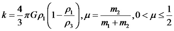
Let the mass of the rigid shell and the second primary be and respectively. Let the density of the incompressible fluid inside the shell be and that of the infinitesimal mass moving inside the shell be and its mass. Let A denote the oblateness coefficient of the first primary such that and the radiation force of the second primary, which is given by such that.

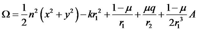
Let and be the centers of m_1, m₂, and m₃ respectively such that and. Let G be the gravitational constant and the coordinates of the infinitesimal mass m. Further, we suppose that the line joining m₁and m₂ is the x-axis. The total potential acting at m is

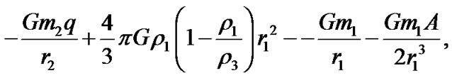
where

The coordinates m₁ and m₂  are and respectively. In dimensionless rotational coordinate system, we choose the unit of mass to be the sum of the masses of the primaries, i.e. and. The unit of length is taken as equal to the distance between the primaries, and the unit is chosen so that.

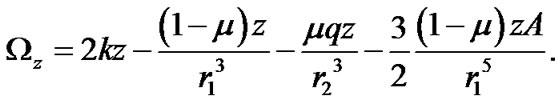
The equations of motion of the infinitesimal body are

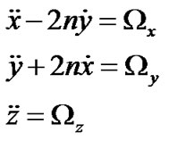(1)

(2)

(3)

(4)

3. Equilibrium Points

Equilibrium points exist for the system when

For (i.e.)

(5)

(6)

(7)

4. Collinear Points

Collinear equilibrium points occur when

and 

The equation

(8)

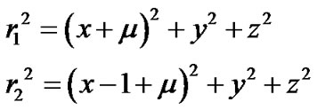
gives the positions of the collinear points. We observe that and so that the collinear points L₁, L₂ and L₃ lie in the intervals (μ,∞), (μ-1,μ) and (-∞,μ-1) respectively.

For L₁, put, and substituting these values of r₁ and r₂ in Equation (8), putting we obtain

(9)

This is a seventh degree algebraic equation in. For both positive and negative values of k there is only one change of sign in the equation. This shows the existence of at least one real root. Similarly, we have for L₂ and L₃

(10)

and

(11)

where are given by Equations (9), (10) and (11) respectively for and. Therefore, the three collinear points are located as

Using MATLAB we generated real roots of the Equations (9), (10) and (11) respectively to compute the respective values of the collinear points.

For constant values of the oblateness factor A and the radiation factor q, there is only one real root of (9) for each = 0,1,3,5 and μ = 0.1,0.2,0.3,0.4,0.5, three real roots of (10) and (11) except for k=1 where there are five distinct real roots in the case of Equation (11).

The variation in values of for various values of the density parameter k and mass parameter μ is shown in Figures 1, 2 and 3 respectively.

In Figures 1-3, the curve k = 0 corresponds to. That is, when the density of the fluid in the rigid shell is same as the density of the infinitesimal mass moving in the shell. The other curves, and correspond to the case when k = 1, k = 3, k = 5 correspond to the case when.

5. Stability of Collinear Points

Let the equilibrium points and their positions be denoted by.Then we substitute

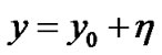and      (12)

into the equations of motion (1) and obtain the equations of variation as

(13)

where and are small displacement in x₀ and y₀ respectively. Retaining only linear terms in and the characteristic Equations of (13) is

(14)

where the superscripts indicate that the partial derivatives of are to be evaluated at the equilibrium points

At the collinear point, so that

and  Therefore,

For values of, 0, A1 the discriminant of the characteristic Equation (14) is positive when k > 0 and negative for k < 0.

Consequently, for k > 0, one root of the characteristic equation will be positive and the other negative, indicating unbounded motion. This makes the collinear

points unstable. For k < 0, both roots of the characteristic equation will complex (imaginary) and indicates oscillatory motion. Hence, the collinear points are stable.

6. Discussion

It is evident from Equations (9), (10) and (11) that the three physical parameters (density, radiation and oblateness) affect the location of collinear points. Using numerical values we obtained nine collinear equilibrium points for our problem (one from Equation (9), three from Equation (10) and five from Equation (11). By keeping the radiation and oblateness factors constant, we observed the variation in the location of the collinear points for various values the density parameter with the mass parameter.

In Figures 1-3, curve k = 0 corresponds to the density of the incompressible fluid in the spherical shell and that of the infinitesimal mass moving in the shell being the same. Curves k = 1, k = 3 and k = 5 correspond to the infinitesimal mass denser than the incompressible fluid in the shell. It is also observed that due to variation of the parameter, keeping radiation and oblateness fixed, the positions of the collinear equilibrium points shifted towards the primaries. Hence, it could be inferred that the three physical parameters have the tendency of moving the collinear points closer to the primaries.

Collinear equilibrium points are generally unstable in classical and some generalized restricted three-body problem. However, it is seen from the discriminant of the characteristic Equation (14) that when the infinitesimal mass is denser than the incompressible fluid in the shell the collinear equilibrium points are unstable and stable when the incompressible fluid is denser than the infinitesimal mass.

7. Conclusions

In studying the stability of collinear equilibrium points in Robe’s restricted three-body problem under the influence of radiation and oblateness of the primaries when the densities of the infinitesimal mass and the incompressible fluid are different nine collinear points were obtained.

The collinear points are found to be stable when the incompressible fluid in the spherical rigid shell is denser than the infinitesimal mass moving in the shell and unstable when the infinitesimal mass is denser than the incompressible fluid.

8. References

[1]       A. AbdulRaheem and Singh, “Combined Effects of Perturbations, Radiation and Oblateness on the Stability of Equilibrium points in the Restricted Three-Body Problem,” Astronomical Journal, Vol. 131, No. 3, 2006, pp. 1880-1885.

[2]       R. K. Sharma, Z. A. Taqvi and K. B. Bhatnagar, Celest. Mech. and Dyn. Astr., Vol. 79, 2001, pp. 119-133.

[3]       J. Singh, Indian J. of Pure and Appl. Math., Vol. 34, No. 2, 2003, pp. 335-345.

[4]       S. K. Shaoo and B. Ishwar, Bull. of Astr. Society. of India, Vol. 28, 2000, pp. 579-586.

[5]       B. Ishwar and A. Elipe, Astrophysics and Space Science, Vol. 277, 2001, pp. 437-446.

[6]       A. L. Kunisyn, Jour. of Appl. Math. and Mech., Vol. 64, No. 5, 2000, pp. 757-763.

[7]       A. L. Kunisyn, Jour. of Appl. Math. and Mech., Vol. 65, No. 4, 2001, pp. 703-706.

[8]       D. V. Schuerman, Astronomical Journal, Vol. 238, 1980, pp. 337-342.

[9]    V. V. Szebehely, Astronomical Journal, Vol. 72, No. 1, 1967, pp. 7-9.

[10]    H. A. G. Robe, Celestial Mechanics, Vol. 16, 1977, pp. 345-351.

[11]    A. K. Shrivastava and D. Garain, Celest.and Mech. Dyn. Astr., Vol. 51, 1991, pp. 67-73.

[12]    C. M. Giordano, A. R. Plastino and A. Plastino, Celest. Mech. and Dyn. Astr., Vol. 66, 1997, pp. 229-242.

[13]    P. P. Hallan and N. Rana, Celest . Mech.and Dyn. Astr., Vol. 66, 2001, pp. 145-155.

[14]    P. P. Hallan and N. Rana, Indian J. of Pure and Appl. Math., Vol. 35, No. 3, 2004, pp. 401-413.