Open Journal of Epidemiology
Vol.3 No.4(2013), Article ID:39629,7 pages DOI:10.4236/ojepi.2013.34023
Cumulative logit model in the analysis of endometrial cancer under a matched pair case-control design
![]()
Epidemiology and Medical Statistics Unit, College of Medicine & Health Sciences, Sultan Qaboos University, Muscat, Oman
Email: ganguly@squ.edu.om, drss.ganguly@gmail.com
Copyright © 2013 Shyam S. Ganguly. This is an open access article distributed under the Creative Commons Attribution License, which permits unrestricted use, distribution, and reproduction in any medium, provided the original work is properly cited.
Received 23 July 2013; revised 23 August 2013; accepted 30 August 2013
Keywords: Logistic Model; Matched Pairs Case-Control Design; Odds Ratio; Ordinal Response; Regression Analysis
ABSTRACT
Background: Binary as well as polytomous logistic models are widely used for estimating odds ratios when the exposure of prime interest assumes unordered multiple levels under matched pairs case-control design. In our previous studies, we have shown that the use of a polytomous logistic model for estimating cumulative odds ratios when the outcome (response) variable is ordinal (in addition to being polytomous) under matched pairs case-control design. The cumulative odds ratios were estimated based on separate fitting of the model at each of the cutpoint level as compared to less than equal to that level. In this paper we propose an alternative method of estimating the cumulative odds ratios and reanalyze the Los Angeles Endometrial Cancer data in the context of dose levels of conjugated oestrogen exposure and development of endometrial cancer under the matched pair case-control design. Methods: In the present study, the cumulative logit model is fitted using a single multinomial logit model for the data. For this, the full maximum likelihood estimation procedure is adopted. A test for equality of the cumulative odds ratios across the exposure levels is proposed. Results: The analysis revealed that there is a strong evidence of risk for developing endometrial cancer due to oestrogen exposure above each of the three dose level as compared to less than equal to that level. The estimated values at the three cutpoint levels were found to be 6.17, 3.60 and 5.16 respectively. Conclusions: The odds of developing endometrial cancer are very high for the users of any amount of oestrogen, even if it is the least dose, as compared to the non-users.
1. INTRODUCTION
In clinical and epidemiological studies, often we carry out matched-pairs case-control design for establishing relationship between an exposure variable and a health outcome. Usually, the measure of association is the odds ratio (OR) [1-3]. The logistic regression model [4] has been widely used in the estimation of ORs in matched pair case-control retrospective designs when the response variable is binary [5-8].Holford et al. [7] proposed a coding method and estimated ORs for nominal and ordinal outcome categories using a binary logistic model with conditional likelihood procedure. Ganguly and Naik-Nimbalkar [9] proposed a method for estimating ORs modeling the retrospective probabilities, when the outcome of prime interest has more than two unordered levels using polytomous logistic model under a pair-wise matched case control design. In that analysis the responses in each group were compared with responses in a control group.
While analyzing polytomous response data, sometimes we encounter a situation in which the risk factor of interest has more than two levels with a natural ordering. Such ordinal response variables usually occur either in the form of “group continuous” or “assessed ordered”. Group continuous responses arose when outcome categories represent contiguous intervals on a continuous scale. For example, consider the data set in Table 1 for 59 matched pairs, extracted from Los Angeles endometrial cancer study, as given in Breslow and Day [10]. While carrying out the analysis they considered the following four ordered levels of estrogen exposure categories: 1) none; 2) 0.1 - 0.229 mg; 3) 0.3 - 0.625 mg; and 4) 0.626 +mg. ORs corresponding to the three dose levels versus no exposure were estimated [10].
In Table 1, the oestrogen exposure may be considered as “tolerance” of the individual and which may be assumed to have a continuous distribution in the population. These tolerances themselves are not directly observable
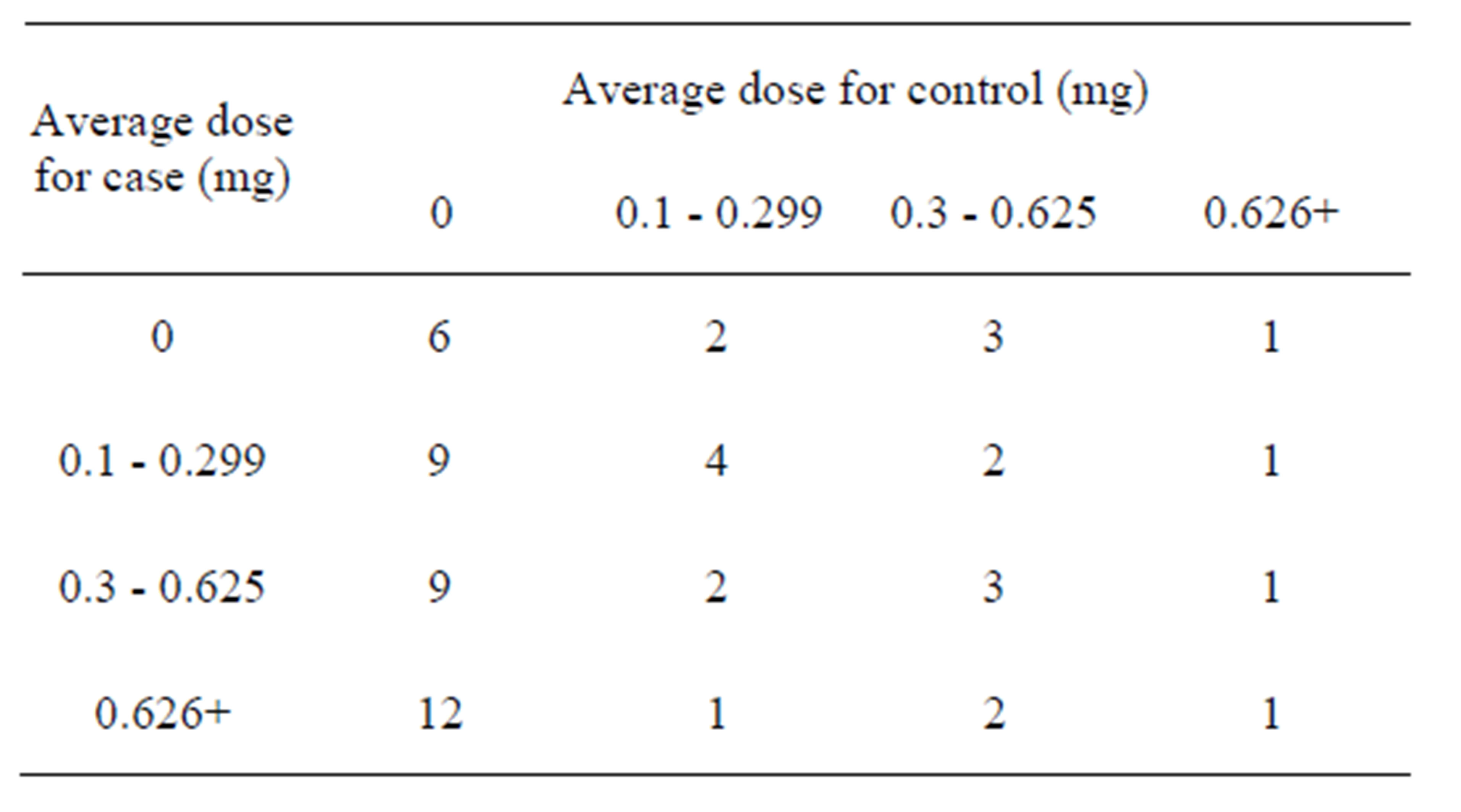
Table 1. Average doses of conjugated oestrogen used by cases and matched controls: Los Angeles endometrial cancer study. (Source: Breslow and Day, 1980).
but decreasing tolerance manifest through an increase in the chances of developing endometrial cancer. Moreover, the categories so formed are contiguous intervals on the continuous scale. Assessed ordered response variable arise from a qualitative assessment for example, while establishing relationship between tonsillar size, which is classified into three ordered categories: not enlarged, enlarged and greatly enlarged, and whether a child is a carrier of the virus streptococcus pyogenes as mentioned by Andorson [11]. In order to carry out the analysis in the above situations, it is necessary to assign scores to the levels of the ordinal variables. In the case of group continuous variable, the scores are equally spaced whereas for the assessed ordered situation the distance between the two scores may not be equal. However, the present communication is restricted to the grouped continuous situation only.
McCullagh [12] and Agresti [13,14] have suggested that when the levels of the risk variable have some ordered structure it is sensible to estimate the ORs in a way that takes into consideration the existence of an underlying continuous and unobservable random (latent) variable. This can be done by grouping the categories that are contiguous on the ordinal scale. Several regression models for the analysis of ordered categorical data have been proposed recently [12-15]. However, despite the growing number of models appropriate to ordinal data, little work has been reported in the filed of matched designs.
In this paper, we describe an alternative method for estimating the ORs, when the response variable is ordinal in nature using cumulative logits and continuationratio logits as suggested in Agresti [13,14] under a pair wise matched case-control design. The approach is based on fitting the full logit model as described in Aitken et al. [16]. We also present an asymptotic distributional result for testing the trend of cumulative OR as the tolerance of the dose levels decreases over the categories.
2. METHODS
2.1. The Models
The model building strategies for ordinal logistic regression model under pair-wise matched case-control design has been elaborated in our previous papers [17,18], however, for the convenience of the readers we describe, in brief, the procedure as follows.
Suppose that the ordinal exposure variable F is a response variable forming k ordered categories and D represents a dichotomous disease condition of an individual, with value 1 if the individual is a case otherwise it is zero. Also when D = 1, F is represented by F1 and for D = 0, F is represented by F0. Let  be the number of observed case-control pairs in the (i,j) the cell corresponding to exposure level of case and exposure level of control, the results of the matched pair casecontrol investigation, with k ordered exposure categories, may be represented as shown in Table 2.
The case-control observation in Table 2 can be collapsed into (k - 1) table of order 2 × 2.
Hence, at the  the k ordered response categories might be represented by a table of the form as given below.
| Control (F0 ) | |||
|
|
| ||
| Case (F1) |
|
|
|
|
|
|
| |


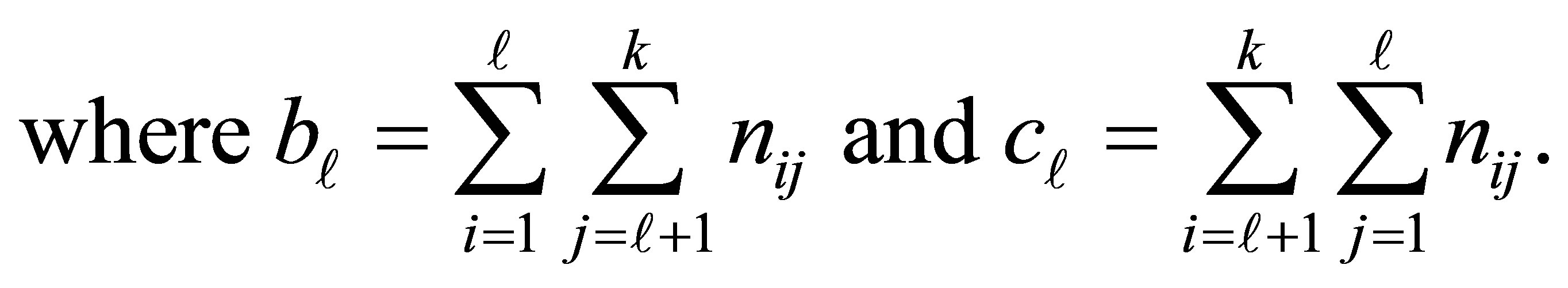
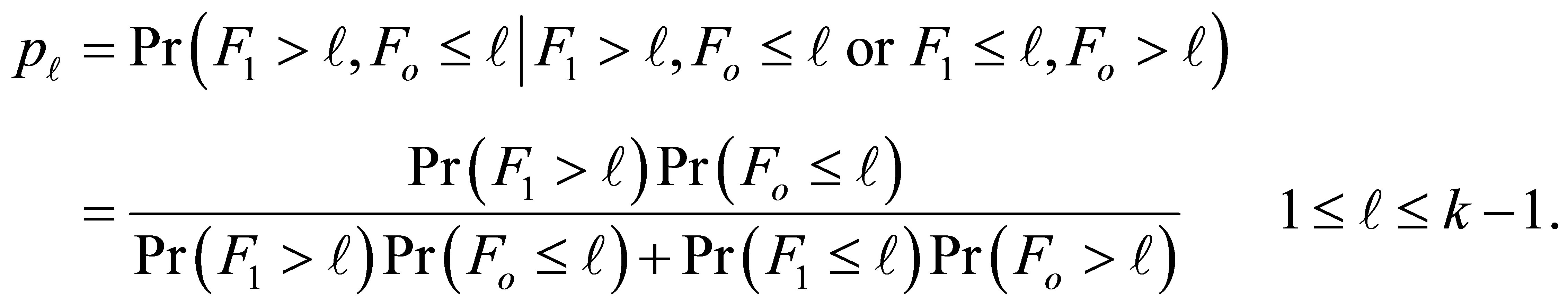
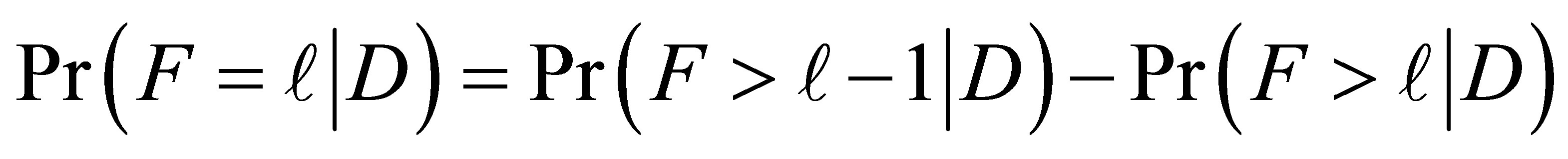
In this situation, the conditional probability that the case responds in a category above  and the control responds in category
  or below, given that the pair is discordant and either the case or the control responds in a category above
  is given by
 (1)
(1)
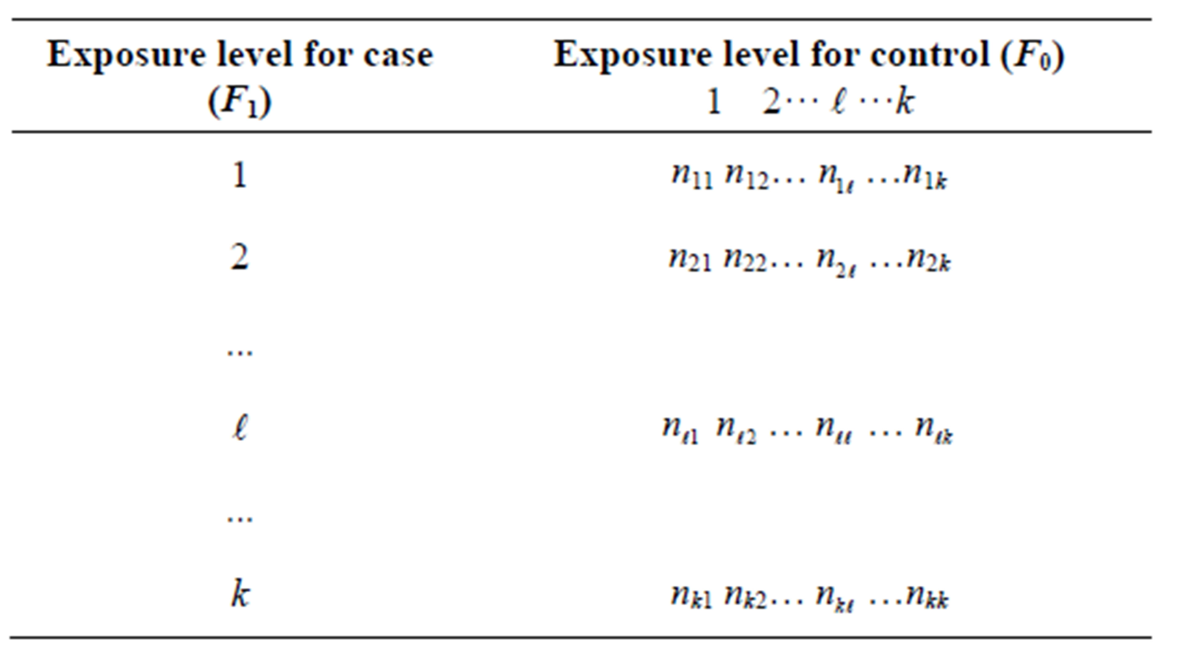
Table 2. Representation of data from a matched pair study with k ordered exposure levels.
We define 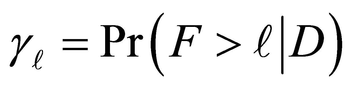 to be the cumulative probability that an individual is classified above exposure level
  under the disease condition D. Then the
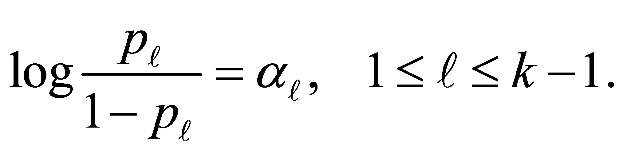
  cumulative logit [12-14] is given by
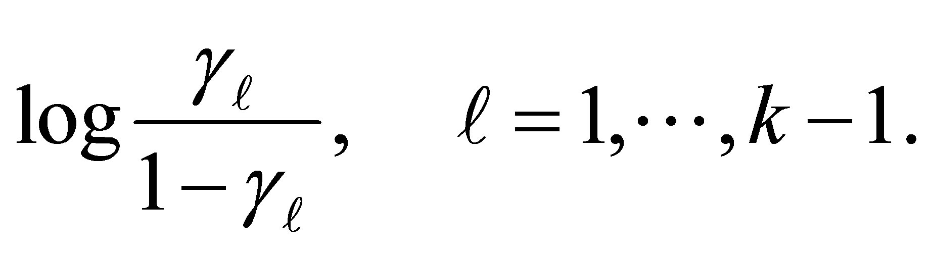 (2)
(2)
A model for cumulative logit (2) is an ordinary logit model for a binary response in which categories 1 to  form a single category, and categories
  to k form second category.
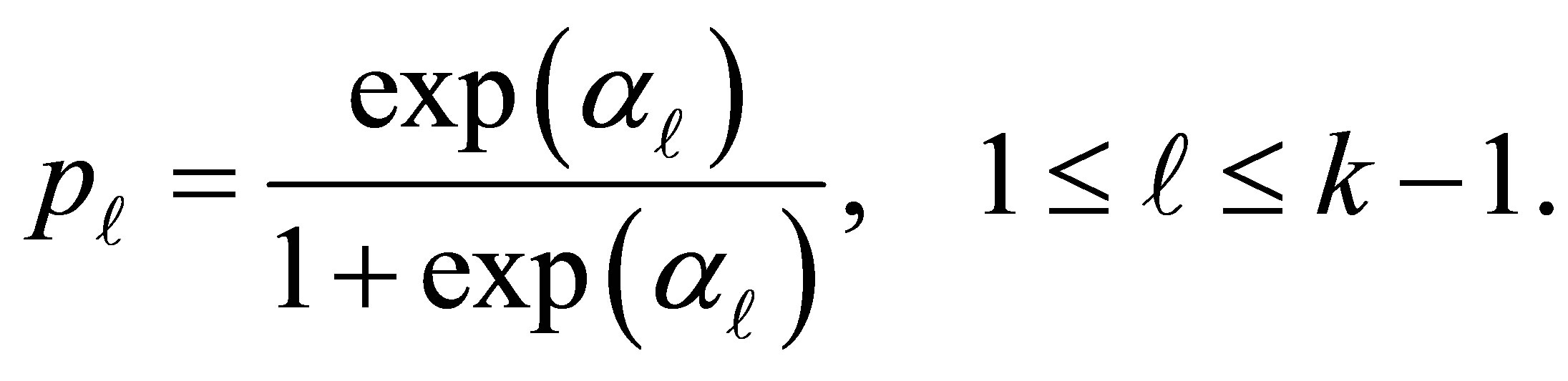
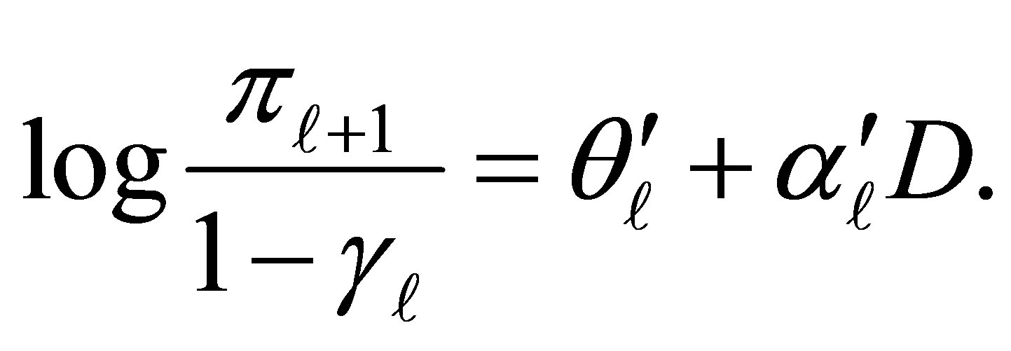
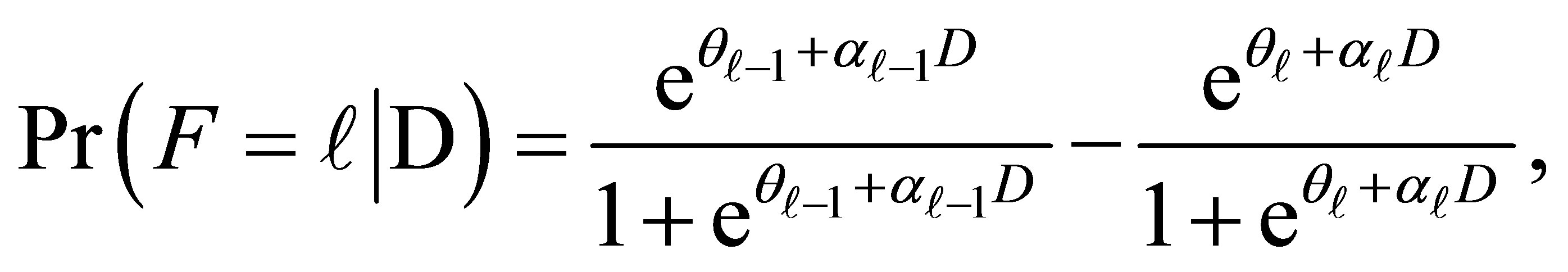
The cumulative probabilities may be modeled [12,14, 15] directly using the cumulative logit link function (2) and may be represented by
 (3)
(3)
Both  and
and 
 in (3) are unknown parameters. Here
  is the intercept or cutpoint parameter and must satisfy
  explains the additional exposure for an individual being classified above the
  level. Using relations (1) and (3), the conditional probability
  is written as
 (4)
(4)
The probability  dose not depends on
 . From (4) we can estimate the “cumulative” log OR for developing the disease for an individual with exposure level more than
  relative to one less than or equal to
 . This is given by
 (5)
(5)
If we consider that the response categories are of interest in themselves, then one can combine the adjacent categories for estimating cumulative ORs. In such a situation the “continuation-ratio” logit link function may be used [13,14], which is given by
 (6)
(6)
where , the response probability of an individual with disease status D, being classified in the
  category
Applying a similar technique, as in the case of cumulative logit link function (2), “continuation-ratio” logit link function (6) may be represented by
 (7)
(7)
In this situation  has a similar interpretation as in the case of
  in model (3) and
  explains the additional exposure for an individual being classified at the
  level as compared to less than or equal to the
  level.
2.2. Fitting the Full Logit Model
The cumulative logit model (3) may be fitted using a single multinomial logit model for the data given in Table 1. For this, the full maximum likelihood estimation procedure as given in Aitkin et al. (p. 240) [16] is adopted. Considering the cumulative probability  the category exposure probabilities can be represented as
 (8)
(8)
The category probabilities (8) under the cumulative logit model (3) is given by
 (9)
(9)
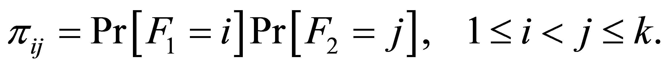
Let  be the probability that for a given case-control pair the case is classified in the i-th level and the control in the j-th level, then the cell probabilities
 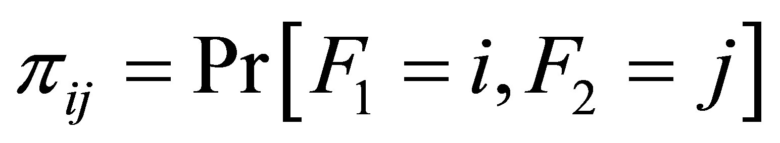 is written as
 (10)
(10)
The full likelihood for the data shown in Table 1 is derived using the multinomial distribution as given below.
The probability that in a sample of N case-control pairs, we observe nij pairs, corresponding to the (i,j)-th cell, is  which is,
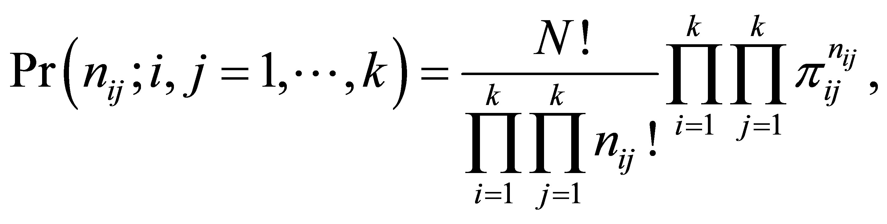 (11)
(11)
with 
Note that there are  distinct probabilities in our case. The estimation and the testing procedures based on the above model are described in brief in Appendix.
The estimated values of cumulative ORs  are obtained using the estimators
  The estimates are written as
 (12)
(12)
The asymptotic variances of the estimated cumulative ORs are obtained by the use of the delta methods [19] and are given by
 (13)
(13)
2.3. Testing of Odds Ratios
In order to examine whether the cumulative ORs (12), based on the full likelihood, procedure are essentially the same, we test the null hypothesis Ho: 
Denoting , then using the properties of ML estimators it can be shown that
  has an asymptotic multivariate normal distribution with
  and with covariance matrix
  Based on the estimated
 ,
,  is obtained. The test of the null hypothesis Ho:
  is equivalent to a test of the liner hypothesis of the form Ho:
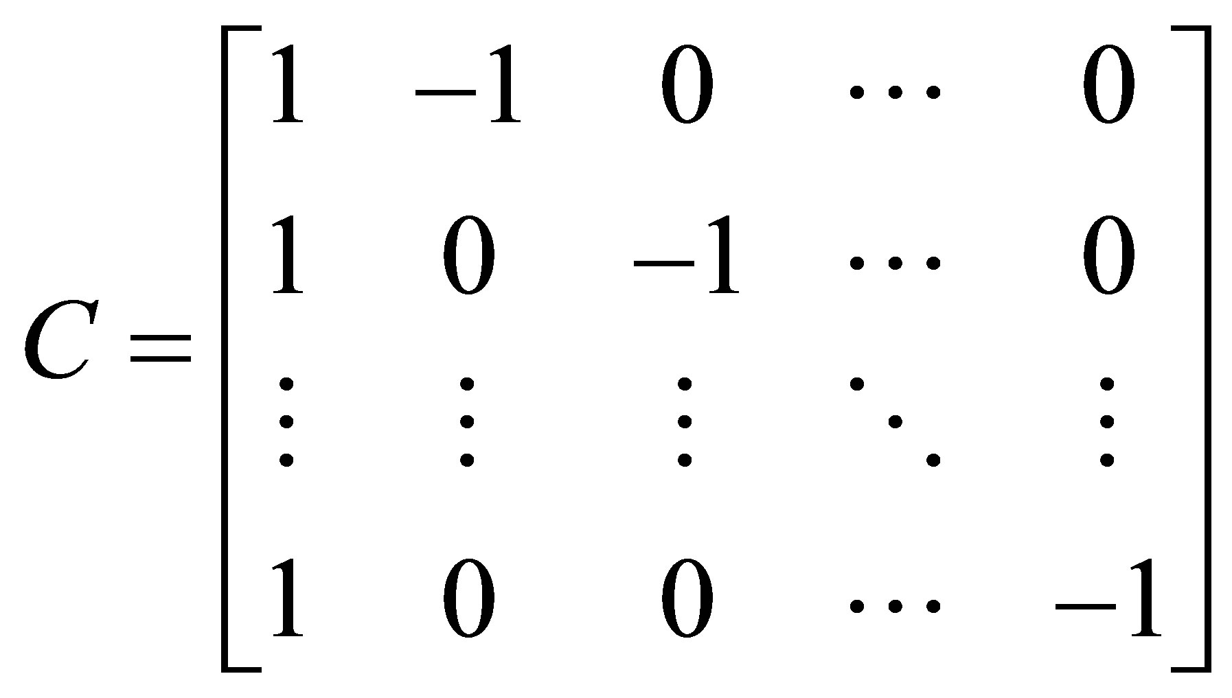
 , where C is a known full rank contrast matrix of order
  and is given by
The null hypothesis is tested using the Wald type test statistic [20], which is given by
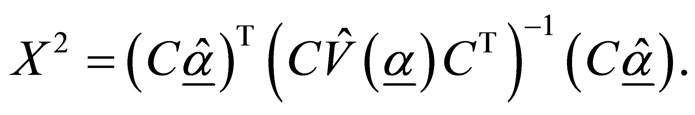 (14)
(14)
Under Ho, X2 is asymptotically distributed as chisquare with degrees of freedom equal to the number of rows of C. If X2 is found significant, individual differences  may be considered to be present indicating the existence of differences of cumulative ORs across the cutpoints.
2.4. Numerical Example
The analytical procedure described above for estimating cumulative and continuation-ratio ORs, for matched pair data with ordered multiple level response categories, is now illustrated by reanalysis of the data set on endometrial cancer given in Table 1. For this data, the marginal totals may be summarized as shown in Table 3.
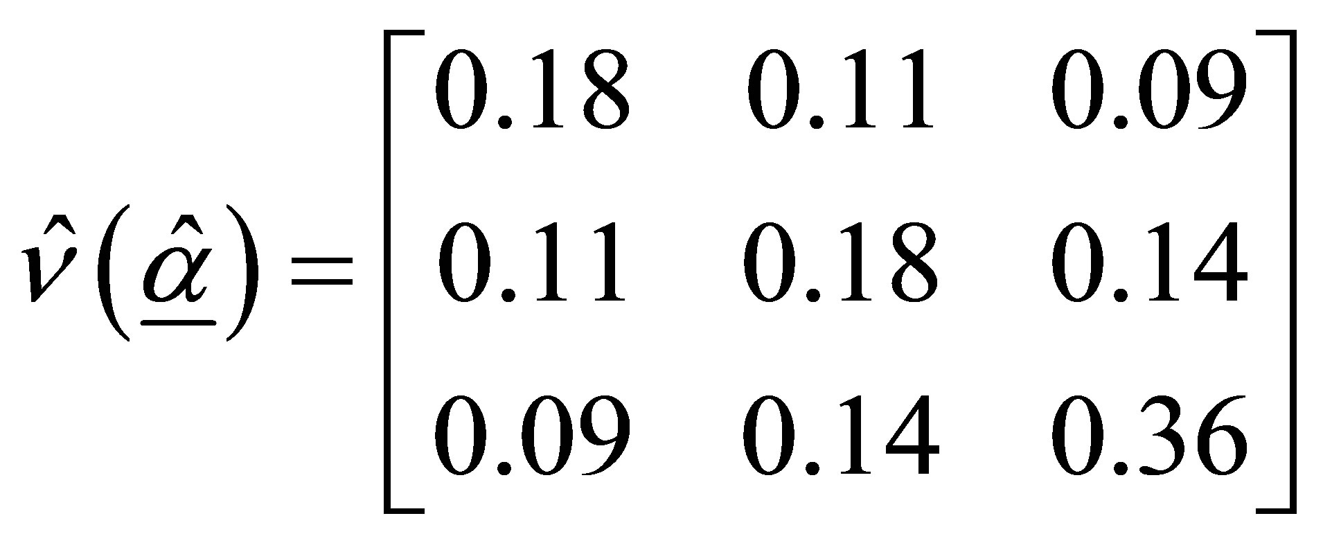
Based on relation (17), the estimated asymptotic covariance matrix  is obtained as:
The maximum likelihood estimates of the parameters  and
and  (i = 1,2,3) with their standard errors, under the cumulative logit model (3) based on full likelihood method is presented in Table 4.
In order to test the validity of considering the i-th cutpoint in the estimation of ORs, the null hypothesis  is tested using large sample Wald chisquare test. The “test-statistic” is found to be significant for
  This shows that, at each cutpoint, there is a strong evidence of risk for developing endometrial cancer due to the higher oestrogen exposure.
Since at each of the three categories, the evidence of risk for developing endometrial cancer is found to be present under the cumulative logit model (3), therefore, based on the estimated values of  cumulative ORs are estimated as shown in Table 5.
In order to test the equality of cumulative ORs across the categories, that is , the null hypothesis Ho:
  is tested using the asymptotic chisquare test (14). The resulting test statistic is found to be 3.70 with 2 degrees of freedom, showing no significant differences between the three cumulative ORs. It may be noted that testing this null hypothesis is equivalent to testing for the McCullagh’s proportional odds model [12].
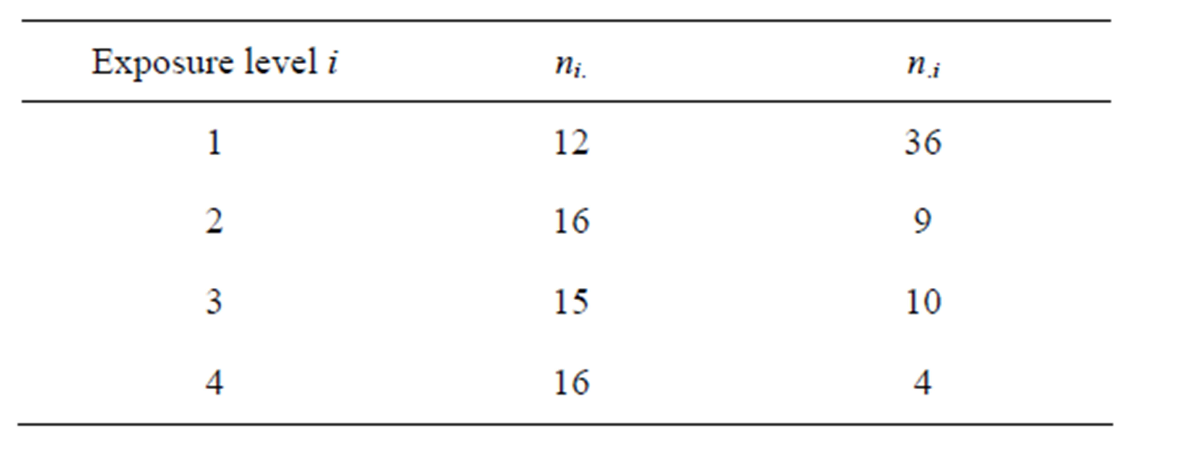
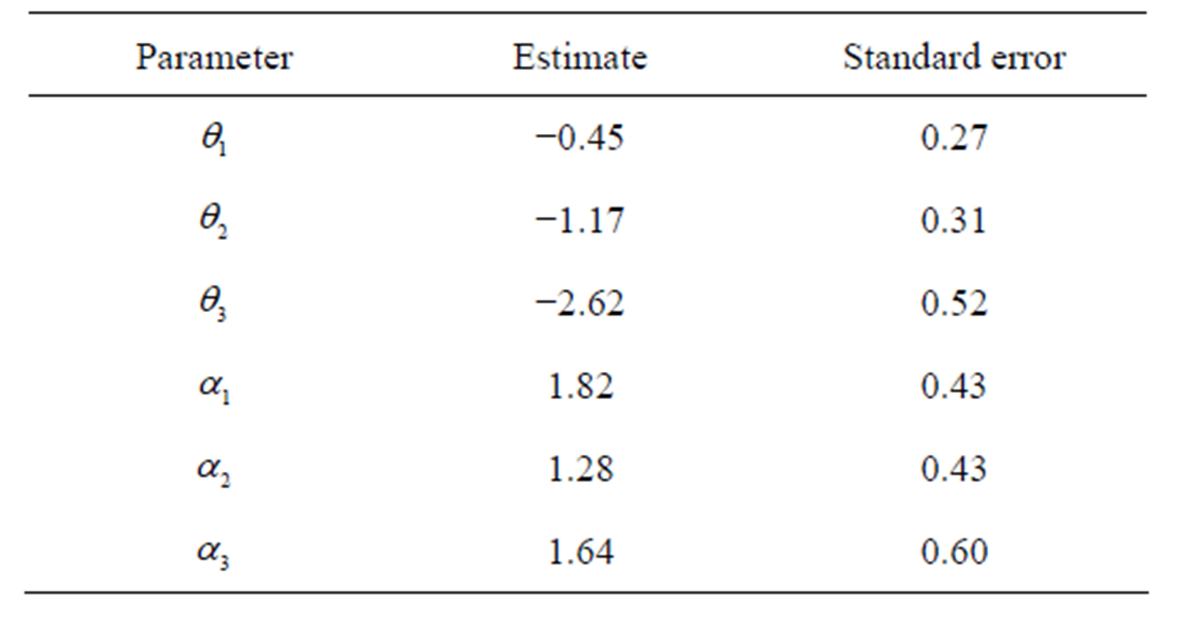
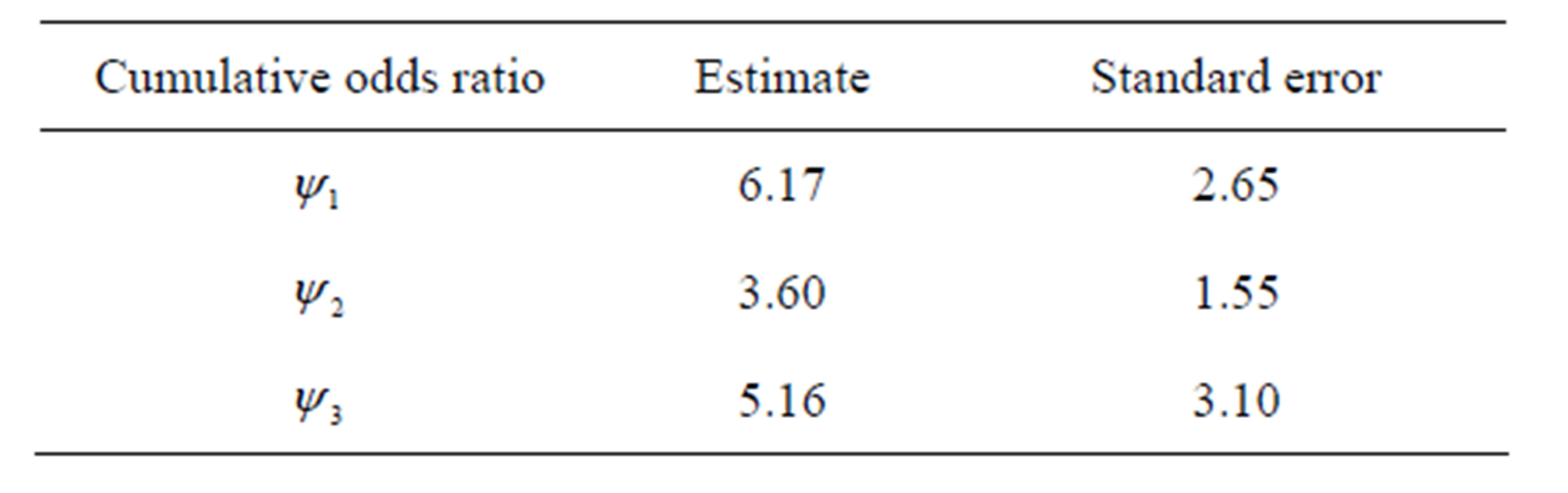
Table 5. Estimation of cumulative ORs at the i-th cutpoint (i = 1,2,3).
Hence, from the above analysis it is observed that although there is a strong evidence of risk for developing endometrial cancer due to the oestrogen exposure above each of the three dose levels as compared to less than or equal to that level, however, their differences are found to be statistically not significant. From this, it may be concluded that the odds of developing endometrial cancer is very high for the users of any amount of oestrogen, even if it is the least dose, as compared to the non-users.
3. DISCUSSION
In recent years, a considerable literature has been accumulated concerning the use of polytomous logistic model for estimating odds ratios, in the development of the disease, in case of a matched case-control design, when multiple case-control groups are considered in the analysis [20-23]. Ganguly and Nik-Nimbalkar [9] suggested the use of polytomous logistic model for estimating ORs, modeling the retrospective probabilities, when the exposure of prime interest has more than two unordered categories, using polytomous logistic model under 1-1 matched case-control design.
Ganguly and Naik-Nimbalkar [17], and further Ganguly [18] extended the concept of cumulative ORs and Continuation-ratio ORs, as suggested in Agresti [13] for ordinal response, to a situation where pairwise matched case-control design is carried out. The method primarily relied on fitting the cumulative logit and continuationratio logit, separately at each cutpoint. In the methods, while constructing the models, the cumulative logit link function at the ith cutpoint (i = 1,2,3) involved the nuisance parameters θi(i = 1,2,3). However, the θ’s get eliminated through the conditionality argument involved in the procedure. Hence, separate fitting of binary logit model provided the estimated values of odds ratios at each cutpoint. The estimated values at the three cutpoints found by Ganguly and Naik-Nimbalkar [17] were 5.00 ± 2.24, 3.43 ± 1.46 and 5.00 ± 1.46 respectively. Interestingly, these values are very close to the results found in the present study.
Breslow and Day [10] have estimated ORs attached to each of the three dose levels of conjugated oestrogen, using the no-dose level as base line. The estimated values of the ORs were 4.59, 3.55 and 8.33 respectively. These ORs measure the risk attached to each of the category relative to the no-dose category. Incidentally, the result found by Ganguly and Nik-Nimbalkar [17] and in the present study substantiates those of Breslow and Day [10]. However, it may be emphasized that the cumulative ORs investigate the behavior of ORs when the subjects have used dose intake more than a particular level as compared to less than or equal to that level. This helps in identifying the dose intake level, which could be regarded as a cutoff point up to which the dose intake may be considered safe.
4. CONCLUSION
In this paper we have presented a method for performing analysis of matched epidemiologic data with an ordered categorical risk factor which explicitly takes account of the ordering by fitting a single multinomial logit model and reanalyzed the Los Angels Endometrial Cancer data given in Breslow and Day [10]. The remarkable feature of the method is that although we estimate the cumulative ORs in the presence of the nuisance parameters but the resulting values found to be very close to that obtained by Ganguly and Nik-Nimbalkar [17] where separate logit models were fitted at each gradation between categories.
REFERENCES
- Mantel, N. and Haenszel, W. (1959) Statistical aspects of the analysis of data from retrospective studies of disease. The Journal of the National Cancer Institute, 22, 719- 749.
- Miettinen, O. (1970) Estimation of relative risk from individually match series. Biometrics, 26, 75-86. http://dx.doi.org/10.2307/2529046
- Ejigou, A. and McHugh, R.B. (1977) Estimation of relative risk from matched pairs in epidemiologic research. Biometrics, 33, 552-556. http://dx.doi.org/10.2307/2529374
- Cox, D.R. (1970) The analysis of binary data. Methuen, London.
- Prentice, R. (1976) Use of logistic model in retrospective studies. Biometrics, 32, 559-606. http://dx.doi.org/10.2307/2529748
- Holford, T.R. (1978) The analysis of pair-matched casecontrol studies, a multivariate approach. Biometrics, 34, 665-672. http://dx.doi.org/10.2307/2530387
- Holford, T.R., White, C. and Kelsey, J.L. (1978) Multivariate Analysis for matched case-control studies. American Journal of Epidemiology, 107, 245-256.
- Kleinbum, D.G., Kupper, L.L. and Chambless, L.E. (1982) Logistic regression analysis of Eipdemiologic data. Theory and practice. Communication in Statistics—Theory and Methods, 11, 485-547. http://dx.doi.org/10.1080/03610928208828251
- Ganguly, S.S. and Naik-Nimbalkar, U. (1992) Use of Polytomous logistic model in matched case-control studies. Biometrical Journal, 34, 209-217. http://dx.doi.org/10.1002/bimj.4710340210
- Breslow, N.E. and Day, N.E. (1980) Statistical methods in cancer research Vol. I. The analysis of case-control studies. International Agency for Research on Cancer, Lyon.
- Anderson, J.A. (1984) Regression and ordered categorical variable. Journal of the Royal Statistical Society: Series B, 46, 1-30.
- McCullagh, P. (1980) Regression models for ordinal data (with discussion). Journal of the Royal Statistical Society: Series B, 42, 109-142.
- Agresti, A. (1984) Analysis of ordinal categorical data. John Wiley & Sons, New York.
- Agresti, A. (1990) Categorical Data Analysis. John Wiley & Sons, New York.
- McCullagh, P. and Nelder, J.A. (1989) Generalized liner models. Chapman Hall, London.
- Aitkin, M., Anderson, D., Francis, B. and Hinde, J. (1989) Statistical modelling in GLIM. Clarendon Press, Oxford.
- Ganguly, S.S. and Naik-nimbalkar, U.V. (1995) Analysis of ordinal data in a study of endometrial cancer under a matched pairs case-control design. Statistics in Medicine, 14, 1545-1552. http://dx.doi.org/10.1002/sim.4780141405
- Ganguly, S.S. (2006) Cumulative logit models for matched pairs case-control design: Studies with covariates. Journal of Applied Statistics, 33, 513-522. http://dx.doi.org/10.1080/02664760600585576
- Serfling, R.J. (1980) Approximation theorems of mathematical studies. John Wiley & Sons, New York. http://dx.doi.org/10.1002/9780470316481
- Prentice, R.L. and Pyke, R. (1979) Logistic disease incidence models and case-control studies. Biometrika, 66, 403-411. http://dx.doi.org/10.1093/biomet/66.3.403
- Dubin, N. and Pasternack, B.S. (1986) Risk assessment for case-control subgroups by polytomous logistic regression. American Journal of Epidemiology, 123, 1101-1117.
- Liang, K.Y. and Stewart, W.F. (1987) Polytomous logistic regression for matched case-control studies with multiple case or control groups. American Journal of Epidemiology, 125, 750-730.
- Hosmer, D.W. and Lemeshow, S. (2000) Applied logistic regression. John Wiley & Sons, New York. http://dx.doi.org/10.1002/0471722146
APPENDIX
In this appendix we derive the log likelihood function for the multinomial logit model and derive the covariance matrix.
The log-likelihood function for k = 4 is obtained using the relation (9) and (10) in (11) which is proportional to
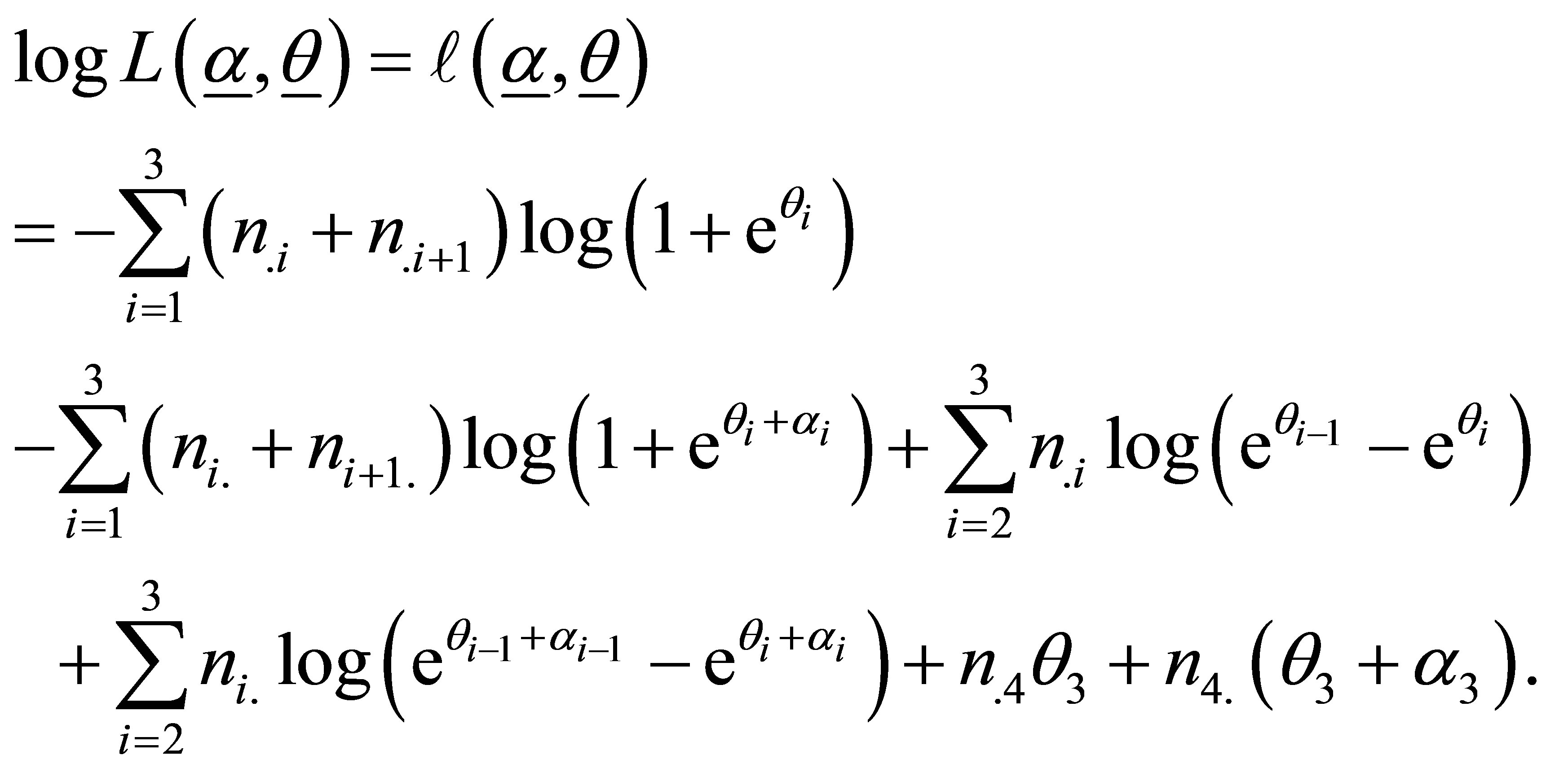 (15)
(15)
where
The log-likelihood function (15) has  free parameters, which are
  i =1,2,3 and
 , i = 1,2 3 respectively.
The likelihood equations are obtained by partial derivatives of  with respect to
  and
and  and are given by
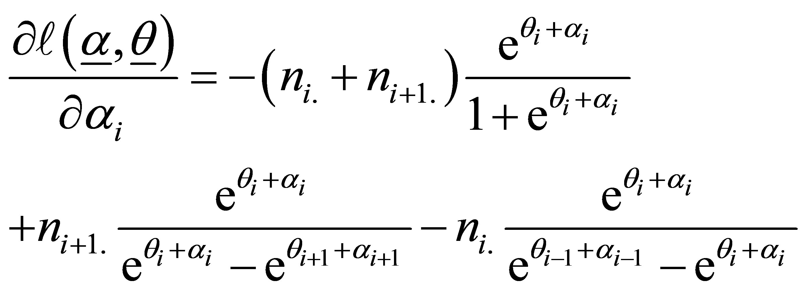
and
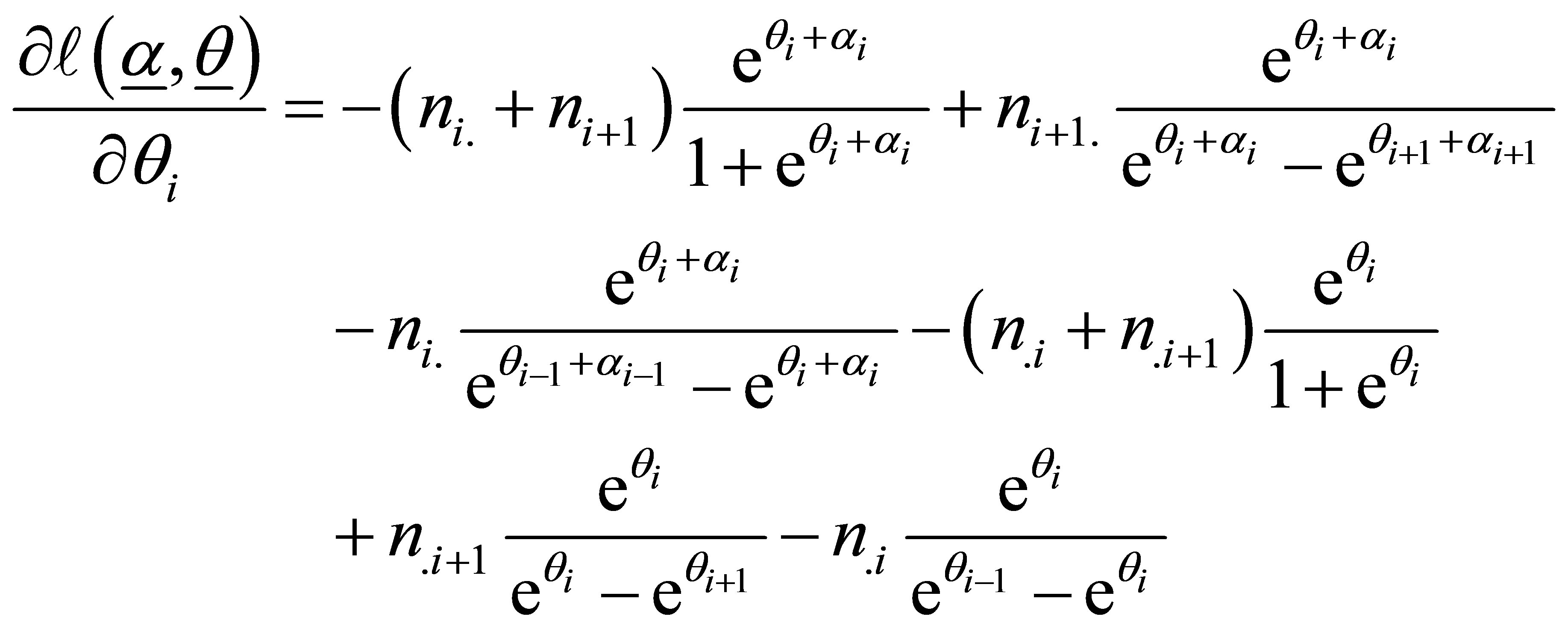 (16)
(16)
For i = 1,
 and
and  are replaced by zero and for i = 3,
 and
and  are replaced by one in (16)
The maximum likelihood estimators,  ,
, (i = 1,2,3) are obtained by setting these likelihood equations equal to zero and solving for
  and
and  respectively. The solutions may be obtained by iterative procedures such as Newton-Raphson method.
The asymptotic variances of the maximum likelyhood estimators  and
and  (i = 1,2,3) are obtained with the use of second partial derivatives of
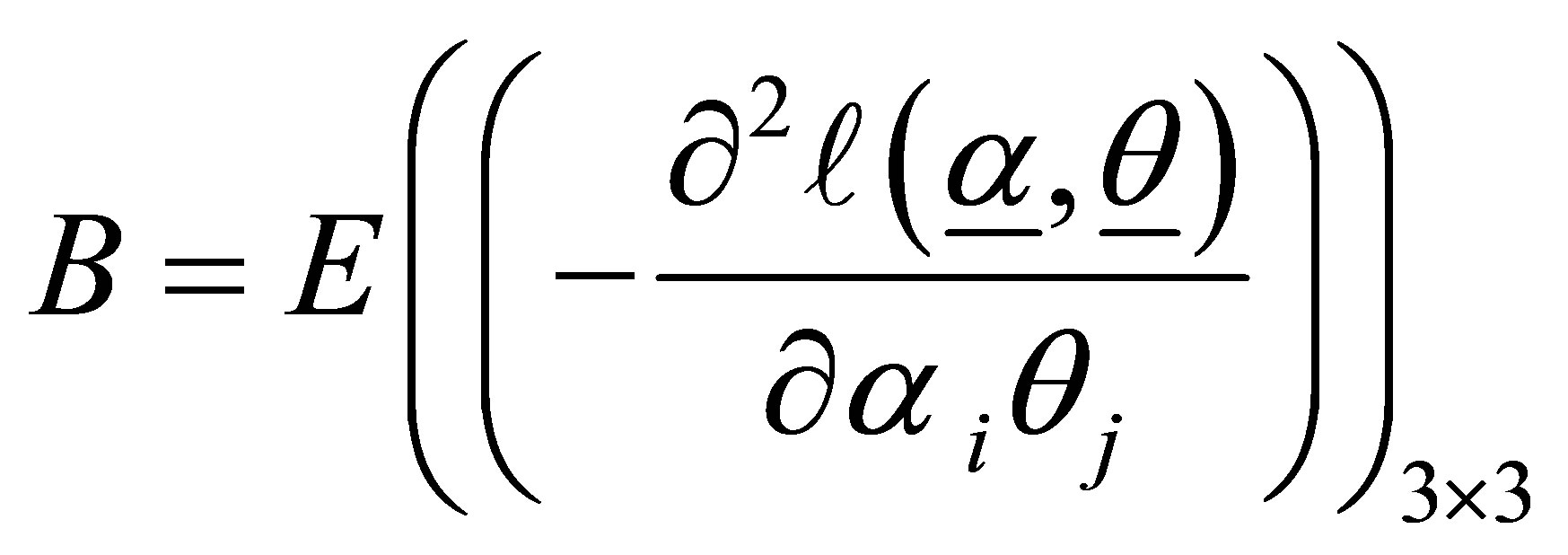
 . The matrix formed by the negative of the expected values of the second partial derivatives gives the information matrix, which may be expressed as the partitioned matrix.
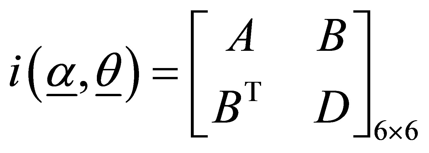 (17)
(17)
where
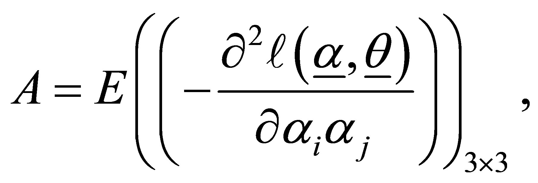
and 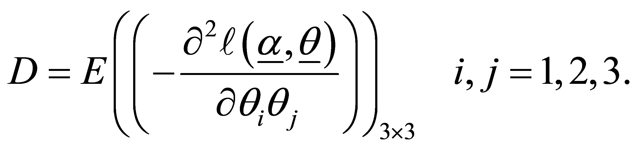
At convergence  provides an estimate of the precision and covariance structure of the estimated coefficients. The estimated standard errors are given by the square roots of the diagonal elements of the matrix