Modern Mechanical Engineering
Vol.3 No.3(2013), Article ID:35736,6 pages DOI:10.4236/mme.2013.33017
Determination of Residuals Stresses Induced by the Autofrettage Treatment by the X-Rays Diffraction Method
1Laboratory of the Electromechanicaly Engineering Badji Mokhtar-Annaba University, Annaba, Algeria
2Laboratory of the Mechanical Systems, Path, Engineering of the Mechanical Systems, Option Structure and Production Ministry of the National Defense, School Military Polytechnic EMP, Alger, Algeria
Email: benretem_a@yahoo.fr, naza_zera@yahoo.fr
Copyright © 2013 Naziha Zerari et al. This is an open access article distributed under the Creative Commons Attribution License, which permits unrestricted use, distribution, and reproduction in any medium, provided the original work is properly cited.
Received March 18, 2013; revised June 17, 2013; accepted June 30, 2013
Keywords: Autofrettage; Elasto-Plastic; Residual Stresses; X-Rays Diffraction
ABSTRACT
Some meaningful advances have been made these last years to value precise and reliable way the residual stresses experimentally created by the autofrettage. The autofrettage process is used widely to introduce residual stresses into thick walled tubes; traditionally residual stresses have been measured using the Sachs method destructive or non-destructive methods. In this paper we describe the application of the X-rays diffraction; this technique permits to justify the presence of the compressive tangential residual stresses, and to value their distribution after two different autofrettage internal pressures loading. The results show that there is a large difference in the residual stresses find in the different autofrettege pressure. One can see the influence of the autofrettage’s pressure quantity on residual stresses created in the thickness of the test tubes.
1. Introduction
The mechanical piece fatigue behaviour or a structure have a strong historic with the solicitations that it undergoes during manufacture processes and during the service hours, under some working conditions. The residual stresses led by these loadings have a big influence on the life of fatigue [1,2]. The residual stresses in the mechanical pieces can result from a lot of sources, residual stress can raise or lower the mean stress experienced over a fatigue cycle. In general, we can classify them like being the harmful stresses that accelerate the starting phases of fatigue growth creeks. In other case, some additional treatments are added after the manufacture process in the specific object to produce some repressive residual stresses beneficial to the most critical structure places. It is now established that the majority of the fatigue failings can be avoided by compressive efforts [3].
This means that considerable advantage can be gained by engineering a compressive inplane stress in the near surface region, for example, by peening, autofrettage into thick walled tubes [4,5].
2. Hydraulic Autofrttage Principle
The basic principle of the hydraulic autofrettage process consists to recharge a thick cylinder by an internal pressure superior to the service pressure. If the internal pressure increases in a thick cylinder, the distortion imposed to the material cylinder is first merely elastic until the elastic limit is reached. Beyond this pressure zone (a), occurs an irreversible plastic distortion zone (b). When the internal pressure is freed after the autofrettage process (discharge), it appears two different layers along the thickness cylinder (a) and (b). The internal, deformed layers plastically, prevent the return elastically in the state of balance the deformed external layers. The thickness of the cylinder undergoes residual stresses in the external layers and compression on the internal layers [6]. These are going to be added algebraically to the stresses to generate by the ulterior application of the service pressure.
3. Determination of the Residual Stresses
3.1. Introduction
A Several methods for the determination of the residual stresses exist currently; we can classify them in destructive or non-destructive methods. Let’s mention among the non destructive methods, the X-rays diffraction and the neutrons diffraction. The destructive methods, for example, the holes method, that requires a drilling to measure the evolution of the residual stresses according to the depth of the holes pierced [7-9]. Let’s recall that the residual stresses are ordinarily divided in three categories:
• Residual stresses I type: macrostresses, i.e. Constant over a large number of grains.
• Residual stresses II type: constant over a single grain.
• Residual stresses III type: constant over the atomic.
What follows is concerned only with residual stresses of the first type (I) [10].
3.2. Bragg’s Law and Diffraction
Bragg diffraction occurs when electromagnetic radiation or subatomic particle waves with wavelength comparable to atomic spacings are incident upon a crystalline sample, are scattered in a specular fashion by the atoms in the system, and undergo constructive interference in accordance to Bragg’s law. For a crystalline solid, the waves are scattered from lattice planes separated by the interplanar distance d. Where the scattered waves interfere constructively, they remain in phase since the path length of each wave is equal to an integer multiple of the wavelength. The path difference between two waves undergoing constructive interference is given by 2dsinθ, where θ is the scattering angle. This leads to Bragg’s law, which describes the condition for constructive interference from successive crystallographic planes (h, k, and l) of the crystalline lattice, as shown in Figure 1. Bragg expressed this in an equation now known as Bragg’s Law:
 (1)
(1)
where n is an integer, λ is the wavelength of incident wave, d is the spacing between the planes in the atomic lattice, and θ is the angle between the incident ray and the scattering planes,  the diffraction angle.
A small change in the lattice parameter  will result in a change
  in the Bragg angle so that the lattice elastic strain is given by:

Figure 1. Bragg’s law.
 (2)
(2)
The diffraction angle sample  is near to 90˚, for which one gets a good compromise between the spatial resolution and the measure precision. The
  angle defines the measure direction on the surface of the sample while the angle
  defines the internal angle there between the normal to the sample and the normal to the diffracting plan. L and P are respectively the reference marks of the laboratory (reference mark of the measure as shown in Figure 2) and of the sample. From the mechanics laws of the continuous surroundings (Hooke laws generalized) and while supposing the homogeneous elastic and isotropy material.
3.3. Measurement of Residual Stresses Using X-Ray  Method
With the homogeneous material hypothesis, macroscopically isotropy and the sufficiently small grains propertied on a plane surface, we can make the stresses calculation [8]. You can use the X-rays diffraction to determine the residual Strains (macrostrains) presented on the surface, in the crystalline material [10,11].
The  method it consists to measure the distance variation between the plans atomic d of a same family.
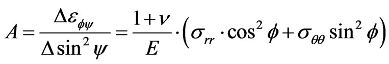
Usually in X-rays diffraction, one considers the superficial measure and with stresses plan state of the materials area with a stresses plan state to the material surface. . This is a base equation for the
  method as follows:
 (3)
(3)
where the main stress directions are unknown, the distributions of lattice strain should be recorde in to two variable directions  and
and . As
. As  = 0˚ - 90˚, Step is 3˚ and
  = 0˚ - 180˚ with 1 and 5 step.

Figure 2. Coordinates systems and notations usually used in strains measure by diffraction. L and P are respectively the reference marks of the laboratory (reference mark of the measure) and of the sample.
 (4)
(4)
 (5)
(5)
 (6)
(6)
 (7)
(7)
3.4. Materials and Sample
The chemical composition of the sample is aluminum alloy (AU4G) given in the Table 1. A schematic of the simple is shown in Figure 3.
These mechanical properties sum up as follows:
• The limit elastic σ0 = 100 N/mm.
• The Young’s modulus E = 74000 N/mm2.
• The tangent modulus Ep = 26,000 N/mm2.
• Poisson’s ratio .
.
• Internal diameter a =30 mm.
• External diameter b = 50 mm.
• Length of sample L = 300 mm.
• The wall thickness K = b/a =1.66.
Equipment for field measurement of residual stresses by X-ray diffraction was performed in the Laboratory Materials, Minerals and Composites (LMMC), University of Boumerdes ALGERIE. Table 2 gives the Operating condition.
3.5. Samples Preparation
For a faithful determination of the residual stresses led by the autofrettage process, it is necessary to eliminate all residual stresses that exist before in the sample tube. By a recook in 530˚C during one half hour, the existing stresses led by the manufacture processes have been eliminated. We consider a thick cylinde, constituted of a

Table 1. Chemical composition table of the tube test.

Table 2. Operating condition of X-rays test.
material considered elasto-plastic to the springiness linear isotope and having for criteria of malleability the one of Trescas or Von-Mis. Leaving from the initial state, this cylinder is submitted to a pressure interior P that one makes grow from scratch while the outside pressure is negligible.
4. Results and Discussions
4.1. Residual Stresses Analysis Produced by Autofrettage Pressure 580 Bars
After The thick tube recharging by an internal pressure the position measure a peak that translates the macroscopic state stresses in the material is accompanied by a distance measure d interreticulaire. These sizes permit to characterize the macro-strains material state. The diffraction measure results after the autofrettage pressure treatment equal to  are regrouped in the Table 3. The d0 value of the AU4G material in the Free State (without strains d0 = 4.04 Å. From the Equation (2) one can calculate
 , if one carries the value of the strains
  accord the value of
  Figure 4. After a simplification, we can write Equation (3) as follows:
 (8)
(8)
 (9)
(9)
 (10)
(10)
From the Figure 4 we can get constant B:

To determine  and
and  to solve the set of two

Figure 3. Test-tube.

Table 3. Result rough of measurements of the test of X-ray autofrettage with 580 bars.

Figure 4. Evolution of the deformation according to  (P = 580 bar).

Figure 5. Evolution of the strains according to  (P = 400 bar).
Equations (9) and (10) are necessary. The results obtained are translated into a curve, shown in Figure 6.
We can conclude that after an autofretagge process at 580 bars we note that:
• The tangential residual stresses , are important in the state of compression that in traction.
• The radial residual stresses  is always of constant tractions, with a very weak constant value by contribution to the tangential residual stresses.
4.2. Residual Stresses Analysis Produced by Autofrettage Pressure 400 Bars
Table 4 gives the angular positions of diffraction 2θ and the distances d inters reticular X-diffraction of the autofrettage treatment at pressure equal 400 bars.
In this case, we determine the residual stresses and going to follow the same stages that one mentioned before. We present the strains curve in function of  in Figure 5, when we can find B equal at −0.7106.
Figure 7 gives the radial and tangential residual stresses distribution at autofrettage pressure of 400 bars. By this figure we can conclude that:
• The tangential residual stresses  is more important in compressions that in traction.
• The radial residual stresses  are always of traction, with the same feeble value by contribution to the tangent stresses.
• Figure 8 shown the analysis results of tow thickwalled tube are subjected to different high interna1 pressure which expands it and leaves residual compressive stresses on the surface of the bore. One can see the influence of the autofrettage pressure on the tangential residual stresses quantity created by this treatment. It has been also observed that, if an autofrettage pressure value is exceeded, the residual stresses increase.
5. Conclusions
The X-rays diffraction technique permits to justify the

Figure 6. Distribution of the residual stresses at pressure load (P = 580 bar).
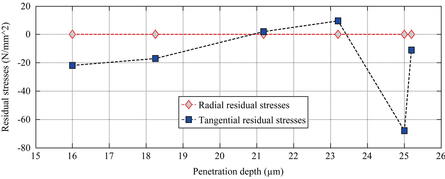
Figure 7. Distribution of the residual stresses at pressure load (P = 400 bar).

Figure 8. Distribution of the residual stresses compared for two different pressures.

Table 4. Result rough of measurements of the test of X-rays autofrettage with 400 bars.
presence of the residual stresses, and to value their distribution.
The results show that the radial and tangential residual stresses distribution find by the X-rays diffraction after an autofrettage test, one can see the influence of the autofrettage pressure on residual stresses created.
REFERENCES
- B. Avitzur, “Determination of Residual Stress Distributions in Autofrettaged Tubing,” International Journal of Pressure Vessels and Piping, Vol. 31, No. 3, 1988, pp. 147-157. doi:10.1016/0308-0161(88)90003-8
- G. A. Webster and A. N. Ezeilo, “Residual Stress Distributions and Their Influence on Fatigue Lifetimes,” International Journal of Fatigue, Vol. 23, Suppl. 1, 2001, pp. S375-S383. doi:10.1016/S0142-1123(01)00133-5
- S. M. Aceves, J. Martinez-Frias and F. Espinosa-Loza, “Certification Testing and Demonstration of Insulated Pressure Vessel for Vehicular Hydrogen Storage,” International Journal of Hydrogen Energy, Vol. 31, No. 15, 2006, pp. 2274-2283. doi:10.1016/j.ijhydene.2006.02.019
- J. M. Alegre, P. Bravo and M. Preciado, “Fatigue Behaviour of an Autofrettaged High-Pressure Vessel for the Food Industry,” Engineering Failure Analysis, Vol. 14, No. 2, 2007, pp. 396-407. doi:10.1016/j.engfailanal.2006.02.015
- H. O. Fuchs, “Techniques of Surface Stressing to Avoid Fatigue,” pp. 197-229.
- J. Faisandier and T. Coll, “Mécanisme Hydrauliques et Pneumatiques,” 8ème Edition, Ecole d’Ingénieur des Arts et Métiers et de Ecole National Supérieur de l’Aéronautique, Paris, 1999.
- D. George and D. J. Smith, “The Application of the Deep Hole Technique for Measuring Residual Stresses in an Autofrettaged Tube,” Proceedings of PVP 2000, Seattle, 23-27 July 2000.
- M. Certiti, “Apport de la Diffraction des Neutron a l’Analyse des Contraintes Interne,” PhD Thèse, Science Chimiques, Université de Paris sud, Centre d’Orsay, 2004.
- M. R. Hill, “Determination of Residual Stress Based on the Estimation of Eigenstrain,” PhD Thesis, Stanford University, Stanford, 1996.
- P. J. Withers and H. K. D. H. Bhadeshia, “Residual Stress Part 1—Measurement Techniques,” Materials Science and Technology, Vol. 17, No. 4, 2001, pp. 355-365.
- G. A. Webster and A. N. Ezeilo, “Residual Stress Distributions and Their Influence on Fatigue Lifetimes,” International Journal of Fatigue, Vol. 23, Suppl. 1, 2001, pp. S375-S383. doi:10.1016/S0142-1123(01)00133-5