ABSTRACT

The exchange option was introduced by Margrabe in [1] and its price was explicitly computed therein, albeit with some small variations to the models considered here. After that important introduction of an option to exchange one commodity for another, a lot more work has been devoted to variations of exchange options with attention focusing mainly on pricing but not hedging. In this paper, we demonstrate the efficiency of the Malliavin derivative in computing both the price and hedging portfolio of an exchange option. For that to happen, we first give a preview of white noise analysis and theory of distributions.

1. Introduction

White noise analysis and theory of distributions is treated extensively in [2-5] and references therein. Applications in the form of the generalized Clark-Haussmann-Ocone (CHO) formula was studied in [6-8] and references therein. The theorem takes advantage of the martingale representation theorem which expresses every square integrable martingale as a sum of a previsible process and an Itô integral. The power of the generalized CHO is that one can take advantage of the Malliavin derivative for computing the hedging portfolio. The Malliavin derivative is a better mathematical operation as opposed to the delta hedging approach whose limitations are a failure to explain differentiation of some payoffs which are not differentiable everywhere or if the underlying security is not Markovian. Most of the attention in contingent claim analysis is directed at pricing because of its importance to market practitioners. It is in this regard that explicit results of hedging portfolios for different options are not always readily available. In this paper, we present both explicit results of the price and hedging portfolio of an exchange option, written on two underlying securities with independent Brownian motions. The ground-breaking work was done in [1]. The market setup is a complete market setup to escape the problem of not finding a perfect hedge.

Hedging portfolios are just as important as prices of options in that they give us an understanding of how sellers or writers can managed dynamically to replicate the payoff of a contingent claim. The price at any time of the contingent claim equals the intrinsic value of the hedging portfolio at that point.In the case of a European exchange option, the payoff is the difference in terminal value of the underlying securities, conditional on the buyer’s terminal asset price being more than the seller’s,. A more interesting problem will be to look at an American exchange option where the buyer would exercise on or before maturity. Such an exercise time will be a stopping time and the price for such an option will be the essential supremum, over all stopping times, of the payoff above. Our attention in this paper is on the European exchange option.

The price of the exchange option will be determined from the CHO formula as the discounted expectation of the payoff while the hedging portfolio will be obtained from the integrant in the martingale representation theorem setup of the the payoff. This integrant involves the Malliavin derivative of the payoff and its market price of risk and in the case that the latter is time-dependent, it reduces to the discounted expectation of the Malliavin derivative of conditioned with respect to the filtration.

Preliminaries

The following is a summary of important results from [6] and [7]. One of the weaknesses of the delta hedging approach is its failure to justify fully the delta because may not be differentiable. Here represents the number of units of stock to be held at any time.

In this setup, if for example , then is not differentiable everywhere. As a result, white noise theory justifies differentiability of in distribution. The differential operator is the Malliavin derivative. This operator is defined in the space of distributions discussed fully in [6] and summarized below.

Let be the Schwartz space of rapidly decreasing smooth functions and be its dual, which is the space of tempered distributions.Now, for and, let denote the action of on, then by the Bochner-Minlows theorem, there exists a probability measure P on such that

(1.1)

where. In this case P is called the white noise probability measure and is the white noise probability space.

As a result, we shall be considering the space, as the sample space, so that our asset prices will be defined on the probability space where is the family of all Borel subsets of. The construction of a version of the Brownian motion then is a direct consequence of the Bochner-Minlows theorem in that if

then clearly and thus

so that immediately we conclude that where is normal with mean 0 and variance. One can easily prove that is really a standard Brownian motion described in [7] as a continuous modification of the white noise process constructed above.

The Brownian motion constructed this way is a distribution and thus special operations like the Malliavin derivative, defined below, are possible. Note that the Brownian motion is not differentiable in the classical sense but is differentiable in the Malliavin sense. The Malliavin derivative is a stochastic version of the directional derivative in classical calculus, with the direction carefully chosen. The following definition is from [7].

Definition 1.1 Assume that has a directional derivative in all directions of the form where for fixed, in the strong sense that

exists in and assume further that there exists such that

, then we say that is differentiable and we call

the Malliavin derivative of.

Just like any operation where using “first principles” is not usually easy operationally, one can use a series of characterizations to the above definition, which includes the chain rule, to compute the Malliavin derivative of any random variable which is differentiable. The set of all differentiable square integrable random variables was denoted by in [7]. As an illustration, we see that and the chain rule yield that,. Here and elsewhere in this paper,.

Therefore classically, one sees that the Malliavin derivative, in some sense, mimics differentiation in deterministic calculus. This is a big departure from Itô derivation which does not in any way make sense as a derivative in classical sense. Thus the space, the sample space, is rich enough to accommodate the concepts we require for our calculations.

The paper is organized as follows: The next section gives the general pricing and hedging formulae for general contingent claims. The next section defines our market model and the final section gives our pricing and hedging results for the European exchange option.

2. General Pricing and Hedging Models in Complete Markets

We now consider the asset prices defined on the filtered probability space where is the standard filtration generated by the Brownian motions, and which is rich enough to represent the information available to traders about all assets on the market at any time.

The first security is a risk-free asset, e.g. bank account where the balance in the bank is and is a solution of the deterministic differential equation

(2.1)

under the assumption of existence of a unique solution. In this case is the interest rate which we shall later assume is constant for computational advantages.

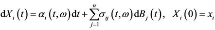
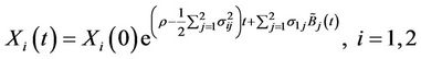
The other securities are risky securities, e.g. stocks where for each, the price of stock number is given by the Ito diffusion

(2.2)

where is the appreciation rate of security number and is the volatility coefficient of the Brownian motion in security.

Let be the vector of appreciation rates for the stocks and the matrix

be the matrix of coefficients of volatility where for easy writing we suppressed dependence on time and noise and the risk factors are modeled by the dimensional Brownian motion

.

Then if, we have

(2.3)

In all these cases we consider for some finite time horizon T and throughout this paper, we are taking to mean transposition.

An investor who selects a portfolio consisting of the assets will have to work out the proportions of his wealth that he has to invest in each of the securities. The vector represents the investor’s holdings at any time, where for each, is the number of units of security number that the investor will hold.

In future we shall refer to the vector of prices as the market and the vector as the portfolio. The holder of a portfolio may decide to liquidate his position at any time, and his wealth is the cumulative savings in the bank account plus the trading gains up to and including the date of liquidation. We assume that the portfolio is self financing, so that, the value of this portfolio at time is given by

The portfolio is called admissible if it is self financing and the value process is bounded below.

We note that by writing the value of the portfolio as and assuming that the portfolio is self financing and admissible, then, if is invertible, we have

where. If we let

, where is the vector of stock prices and if we further assume that satisfies the Novikov conditions, then, by the Girsanov theorem, given by is a Brownian vector with respect to the probability measure given by

.

In this case we are considering as the usual norm in.

Therefore

(2.4)

Solving for we get

(2.5)

From now on, without loss of generality, we assume constant coefficients. Then equation (2.5) becomes

(2.6)

This is a particular version of the Martingale Representation Theorem which can be found for example, in [9] applied to a particular square integrable martingale . It is this Martingale Representation theorem which the CHO formula relies on. We state here the theorem without proof and refer the reader to [6] for more details.

Theorem 2.1 (The generalized Clark-Ocone-Haussmann formula)

Suppose that and assume that the following conditions hold:

1)

2)

3)

then

where is the Girsanov kernel, is the equivalent martingale measure and is a Brownian motion with respect to.

By letting and applying the generalized CHO formula to, we have

(2.7)

where denotes the Malliavin derivative.

By uniqueness due to the Martingale Representation Theorem, we get

(2.8)

and

(2.9)

where as before and means transpose.

Therefore

(2.10)

This gives the explicit number of units of stocks. The holding in the bank account can be found from the self financing condition.

The importance of these results is that in a complete market, every contingent claim with payoff is attainable by a portfolio of stocks and bonds. Therefore, the initial value of a self financing portfolio, equals the price of such a derivative, since . It then shows that the time zero price of such a contingent claim is the discounted expectation of the payoff. Simplifying (2.8) depends on the nature of the payoff. One may directly compute the expectation on condition that the distribution of is known. Sometimes it may be easier to determine the BlackScholes partial differential equation satisfied by the value function with corresponding boundary conditions. If such a boundary value problem can be simplified explicitly, or through numerical techniques, then the price can be determined either explicitly or as a good approximation respectively. Other direct numerical methods of solution like the Monte Carlo simulations involve simulations of the underlying security itself and approximations of the expected values give estimate of (2.8). In this paper, we will find explicit results using some important change of measure transformations which we prove first.

3. The Two Dimensional Market Model and Transformation Theorems

Suppose that traders will agree to trade an option which gives the holder the right, but not obligation to exchange a predetermined risky security with another predetermined risky security, then we call such an option an exchange option. We shall consider the case of a European exchange option. Suppose that the underlying securities in question have time prices and and to simplify our computations, we assume that the market consists of a bank account and these two stocks. The price of the bond is given by (2.1) albeit with constant force of interest. The risky securities are given by

(3.1)

where as before is a standard Brownian motion.

Assume that these stochastic processes are defined on a filtered probability space where is a filtration for the assets such that the stochastic processes are adapted. Suppose that at terminal time, then . Then the payoff of the exchange option will be.

We want to determine the price and the hedging portfolio of this option by using the generalized CHO formula. We assume in our case that the coefficients are constant.

The Girsanov change of measure for this setup can be easily done by letting where;

; and.

Then with constant coefficients, we can easily justify that satisfies the Novikov conditions, so that the probability measure defined by

(3.2)

is equivalent to and is a martingale with respect to. In this case

is a martingale.

Moreover is a Brownian motion with respect to. Let

.

With respect to price is

so that

is a Q-martingale.

In order to exploit the results from the previous discussions, we note here that the market is a special case of the -dimensional market considered in the previous section with n = 2 in this case. We assume that is invertible so that the market is complete. Therefore if we choose a self financing portfolio which is also admissible, then the discounted value of the portfolio at any time is given by

where.

In this case we note that from the CHO formula , for any contingent claim, we get

(3.3)

and

(3.4)

where and

.

Note that since we have assumed that the market is complete, then.

Transformation Theorems

In order to facilitate our computation and taking advantage of the distribution of the terminal values of the underlying securities and, we provide some important transformation results. Their usefulness will be evident in simplifying both (3.3) and (3.4).

Proposition 3.1 Let and be two independent standard normal random variables and let. Define a probability measure equivalent to with density

.

Then the random Gaussian variable and are independent standard normal variables with respect to.

Proof.

We have to prove first that and are independent normally distributed random variables with respect to the probability measure.

Recall that a random variable with mean

and variance is normally distributed if its characteristic function is

In our case we have

Therefore is normal with mean and variance 1, with respect to. Therefore is normal with mean zero and variance 1 with respect to.

In the same way we can show that is normal with mean

and variance 1 since

.

To prove that and are independent with respect to it suffices to prove that and are uncorrelated , that is,.

Now

Corollary 3.1

Let and be as given in Proposition 3.1 and let and be real numbers. Then

where and

Proof.

We have

By using the notation in Proposition 3.1, then the previous expression can be re-written

(6)

We have shown in Proposition 3.1 that the random variables and are standard normal distritions with respect to, so that with respect to the same probability measure, the random variable has a normal distribution with mean zero and variance. In the same way, with respect to, the random variables and are standard normal distributions so that is a normal distribution with mean zero and variance.

Therefore (6) becomes

□

Remark 3.1

Proposition 3.1 still holds in an m-dimensional case where both and are independent multivariate standard normal random vectors. In that case, the following results will be extensions of the preceding proposition and corollary respectively.

Proposition 3.2

Let and be two independent m-dimensional normal random vectors each with mean equal to the zero vector and covariance matrix equal to the identity matrix and let be any non-zero vector. Define a probability measure, equivalent to with density, where is the usual norm in.

Then and are independent Gaussian vectors with zero mean (vector) and covariance matrix equal to the identity.

Consequently Corollary 3.1 can be extended as follows:

Corollary 3.2 Let and be as in Proposition 3.2 and let and be real numbers. If and are m-dimensional vectors, then

where and and denotes the usual norm in.

4. Price and Hedging Portfolio of an Exchange Option

Note that if, for a fixed time horizon, the random variables and in the previous proposition are Brownian vectors and respectively, then the equivalent probability measure will be given by the density and we would also insist that the vector satisfy the Novikov conditions.

We are now ready give the price and hedging portfolio of the European exchange option.

4.1. Price of a European Exchange Option

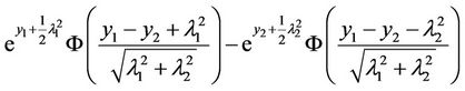
Proposition 4.1 The price of the European exchange option is given by

where is the cumulative distribution function of the standard normal distribution.

Proof.

We had noted that with respect to the equivalent martingale measure which we defined, the prices of the two underlying assets and are given by

where and

.

Therefore the time zero price of the European exchange option is

If we define the probability measure equivalent to by, then

By using the results of the previous proposition, we then conclude that the time zero price of the European exchange option is given by where

and

Note that.

Moreover, since and

, then and ss

so that the time zero price of the European exchange option becomes

Note that this price does not depend on the appreciation rates of the stocks nor on the market interest rate, but just on the market volatilities. This result is also similar to the one obtained in [1] but in that paper the author considers the case when the Brownian motions are correlated and also with a special assumption that the noise terms for each stock are different. We have allowed that stock prices to depend on the two Brownian motions.

4.2. Hedging an Exchange Option

We now calculate the hedging portfolio . For this two dimensional case, thanks to the CHO formula, we get, from (2.9), that

, where, as before

, with and

.

Now

where

. Therefore

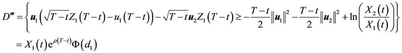
We thus have the following result Proposition 4.2 The perfect hedge is given by

and

where,

and

Proof.

In order to calculate, we need to use the Markov property . We first calculate as follows:

where.

Therefore the previous expression becomes

.

Note that, with respect to, we have

.

Therefore since is independent of then

where

Using the previous notations of and, then the previous expression reduces to

where.

Now, with respect to and for each j = 1, 2 we have is a normal distribution with zero mean and variance then is a normally distributed random vector with mean zero (vector) and covariance matrix equal to the identity matrix. Moreover the previous expression becomes

where

Therefore

with

where

where

In the same way we can also calculate 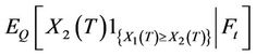to get the result as where

In summary we have

.

Therefore the equation gives

.

Solving for and we get:

and

where.

The number of units in the bond, at any time will be computed from the expression

□

To the best of our knowledge, this result has not been obtained before in its explicit form. However, since the market is Markovian, we could still check this result of the hedging portfolio by differentiating the value function with respect to the stock prices and.

5. Conclusion

We have shown that white noise analysis is of vital importance to Finance in that the generalized CHO formula becomes important in finding explicit expressions for the price and hedging portfolio of European contingent claims. Extensions of these results would be to get similar explicit results when modelling stock prices with general Itô-Lévy processes, though one has to carefully consider the models of prices to avoid incompleteness. Hedging an option is important in that the seller would know how much of each security to hold in order to hedge his liability. In complete markets, this should always be possible and thus the results in this paper can be applied to any European contingent claim. The [1] opened the door for pricing the exchange options though in that paper, the stock prices were influenced each by one Brownian motion and the two were given as correlated. In our case, we allowed the stock prices to each depend on the two noise terms which are independent. Also in our paper, we have computed explicitly, the hedging portfolio, something which was not done in [1]. As a result, our results are extensions of that paper with the strength of using white noise analysis.

6. Acknowledgements

This work was supported by the University of Cape Town Research Grant 461091 .

REFERENCES

- W. Margrabe, “The Value of an Option to Exchange One Asset for Another,” Journal of Finance, Vol. 33, No. 1, 1978, pp. 177-186. doi:10.1111/j.1540-6261.1978.tb03397.x
- T. Hida, H.-H. Kuo, J. Potthoff and L. Streit, “White Noise,” Kluwer, Dordrecht, 1993.
- T. Hida and J. Potthof, “White Noise Analysis—An Overview, White Noise Analysis: Mathematics and Applications,” World Scientific, Singapore, 1989.
- H. H. Kuo, “White Noise Distribution Theory,” CRC Press, Boca Raton, 1996.
- N. Obata, “White Noise Calculus and Fock Space,” Springer-Verlag, Berlin, 1994.
- K. Aase, B. Oksendal, N. Privault and J. Uboe, “White Noise Generalizations of the Clark-Haussmann-Ocone Theorem, With Application to Mathematical Finance,” Finance and Stochastics, Vol. 4, No. 4, 2000, pp. 465- 496. doi:10.1007/PL00013528
- B. Øksendal, “An introduction to Malliavin Calculus with Applications to Economics,” Working Paper 3/96, Institute of Finance and Management Science, Norwegian School of Economics and Business Administration, Bergen, 1996.
- I. Karatzas and D. Ocone, “A Generalized Clark Representation Formula, with Application to Optimal Portfolios,” Stochastics and Stochastic Reports, Vol. 34, 1991, pp. 187-220.
- B. Øksendal, “Stochastic Differential Equations,” 5th Edition, Springer-Verlag, Berlin, 2000.