ABSTRACT

The present article studies the stability conditions of central control artificial equilibrium generalized restricted problem of three bodies. It is generalized in the sense that here we have taken the larger primary body to be in shape of an oblate spheroid. The equilibrium points are sought by the application of the propellant for which it would just balance the gravitational forces. The launching flight of such a satellite is seen to be applicable for having arbitrary space stations for these different missions. Specialty of the result of the investigation lies in the fact that an arbitrary space station can be formed to attain any specified mission.

1. Introduction

An important recent publication on total sailing is a book by Mclnnes [1] which provides a large number of references on the topic. Although solar sailing has been considered as a practical means of space craft propulsion only relatively recently, but the fundamental ideas are by no means new. In 1920s the Soviet father of astronautics Konstantin Tsioslkovsky and his coworker Tsander wrote of using tremendous mirror of very thin sheets [2,3] and using the pressure of sun light to attain cosmic velocities. The concept of solar sailing was reinvented much later by Richard Darwin at the IBM Watson laboratory in New Jersey and he published the first paper on solar sail in journal “Jet Propulsion” in 1958 [4], and he was the first man to coin the word solar sailing. In the early 1970s at the Battelle Laboratories in Ohio [5] discovered a trajectory that could allow a solar sail to comet Hally.

At the initial stage an extremely large (800 m × 800 m) three axis stabilized square solar sail with four deployable booms was considered but was dropped in 1977 due to the perceived risks associated with boom. Nowadays a square solar sail configuration is seen as optimum for these smaller solar sails.

The mission using solar-electric propulsion was initially strongly supported but later on due to escalating cost the propulsion was dropped [6]. The Russian company NPO Energia deployed a spinning 20 m reflector in February 1993 and further refinement of the reflector mission continued. Recently European space agency (ESA) and German aerospace agency (DLR) cofounded the fabrication of a 20 m × 20 m solar sail which was successfully ground tested in December 1999 [7]. After the ground test the agency funded a series of mission studies and later it is being funded in USA and other centers of cosmic research. Looking to future it is being planned to set up a mission to study the various inner and outer planets by means of establishing artificial stations in their neighborhoods.

Solar sail is a proposed form of spacecraft propulsion that takes advantage of the radiation pressure to propel a spacecraft by means of a large membrane mirror. The impact of the photons emitted by the sun on the surface of the sail and its further reflection accelerates the spacecraft. Although this acceleration produced by the solar radiation pressure is smaller than the one achieved by the traditional propulsion systems, this one is continuous and unlimited. This makes long-time missions more accessible [1]. It also opens a wide range of possible mission applications that cannot be achieved by a traditional spacecraft [8].

Sun-sail and other hybrid sails have been recently proposed to explore various cosmic research programmes. An electric sail was proposed to be designed which could be capable of guarantying the fulfillment of trajectories that would be otherwise unfeasible through conventional system. In particular, the proposal [9] was to analyze the electric sail capabilities of generating a class of displaced non Keplerian orbits, useful for the observation of Polar Regions. Secondly earth-escape strategies happen to be an important problem. With growing interest in solar sailing comes the requirement to provide a basis for future detailed planetary escape mission [10] analysis by drawing together the prior work, clarifying and explaining previously anomalies.

The Lagrangian points of the circular restricted problem of three bodies (CR3BP) are known to be the five positions in an orbital system rotating with the two massive bodies where a small object (e.g. a spacecraft) affected by their gravity and centripetal forces can be stationary relative to the two larger bodies. Now if some propellant forces such as solar sail or electrodynamics or magnetic are introduced, then we have some other or more equilibrium points [11] which are artificial equilibrium points or Lagrangian points [AEPS]. The problem of describing the location of AEPS and of investigating their stability property has been studied by several authors. In this connection, the works [12,13] may be specially mentioned, which investigated the effects of the thrust due to the radiation pressure and showed that there are seven equilibrium points and also linear stability was studied. Some scholars [14] by introducing a propellant force acting radially have also shown the existence of seven and more equilibrium points and have examined the stability numerically. Really different studies regarding the effect of the solar sail and the corresponding existence of equilibrium points have been made and in this connection the mention may be made [1,8,10]. The low thrust systems were studied by some scholars [15]. These studies have shown the existence of infinite equilibrium points depending on the magnitude of the propulsive acceleration. However only a subset of the potentially achievable AEPS turns out to be stable and could be used by a spacecraft without the use of a suitable control system. The first proposed the use of a stationary satellite hovering above the earth poles with solar radiation pressure balancing gravitational forces [16]. In 1994 only continuous surfaces of unstable AEPS were derived [10], when low thrust control acceleration was added. It was proved only in 2007 that [15] a marginal stability can be found in a region of space far enough from the second primary. Really the topology of such a subset of stable AEPS is strictly dependant on the propulsion system employed by the spacecraft. It has recently been pointed [17] that for a low propulsive acceleration, the stable AEPS are confined to a very restricted region around the classical Lagrangian points. These artificially generated equilibrium points offer the possibility of considering very interesting mission applications. For example we may take Geostorm warning mission and the Polar observer mission [8]. The Geostorm is a mission concept where a modest sail is placed sunwards of the classical Earth-Sun point. Then with a magnetometer we can detect the solar wind polarity and give enhanced warning of the geomagnetic storms, doubling the time of alert of conventional Halo orbiter such as SOHO. The aim of the polar observer mission is to provide constant viewing of the polar region and could be useful to image the Polar Regions or carry out studies on the climate evolution in the Arctic or Antarctic zone. The present paper presents a generalization of the work [17] in the sense that the formers have taken the shape of the earth to be of a sphere, whereas different from them, we have taken the shape of the earth to be an oblate spheroid. We have followed the same process as in the referred work [17]. Our process differs from that of [17-22] only having mathematical expressions and in our final results. Our work consists of five sections. It starts with a general introduction giving a background of the problem and some progress that have come to our notice and also some applications. The second deals with differential equations of motion and the propellant forces leading to the equilibrium positions, i.e. AEPS. The third section deals with the linearization of the equation of motion in Hamiltonian form. In the fourth section we find out the stability conditions restricting to linear stability alone. In the fifth section we find out minimum controlled artificial equilibrium points and we finally draw our conclusion of the investigation.

The paper has been concluded with the appendices giving the calculations of the various terms occurring in the paper and in the last section a final conclusion of our studies has been given.

2. Equations of Motion

Using dimensionless variables and a system the equations of motion referred to the solution [5,6] when the origin is taken at the smaller mass M₂ may be written as:

(2.1)

where,

R_e = Equatorial radius of the larger mass, R_p = Polar radius of the larger mass, R = 1 = the mutual distance between the primaries.

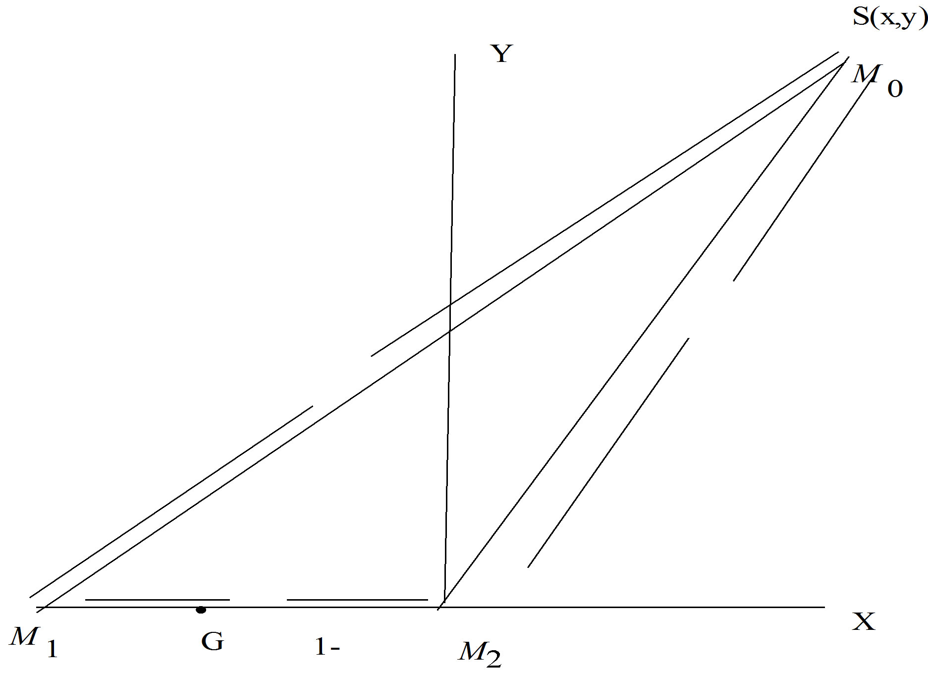
[The larger mass is placed at M₁ and the smaller one at. is their centre of mass and and. The space-craft is taken at M. The line is taken for the X-axis with for the origin and perpendicular at for Y-axis and the axes are taken to be rotating along a normal to - plane with the angular velocity n].

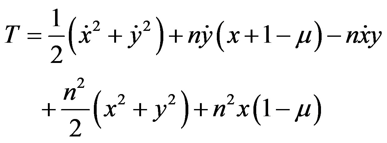
The inertial kinetic energy per unit mass is given by

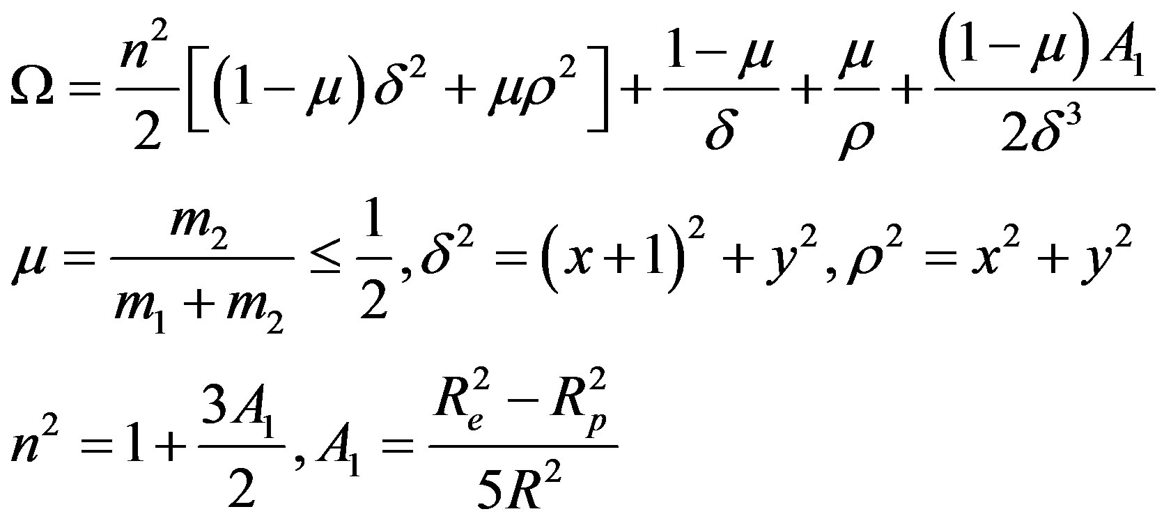
and the total potential due to the gravitational and the control acceleration is:

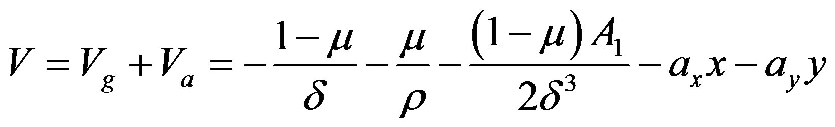
where are the x and y components of the control acceleration. Thus the Equations (2.1) may be written as:

(2.2)

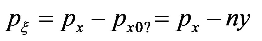
Then the equilibrium point for the control acceleration will be given by

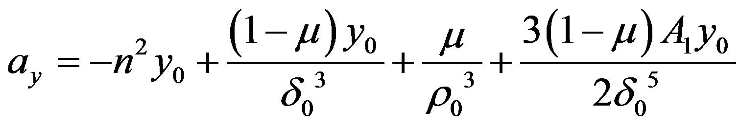
where are the radial distance of the equilibrium point from the primaries.

3. Linearized Equations of Motion Conditions

In this section we shall find out the conditions for the linear stability of the equilibrium points. We have for the Lagrangian function as:

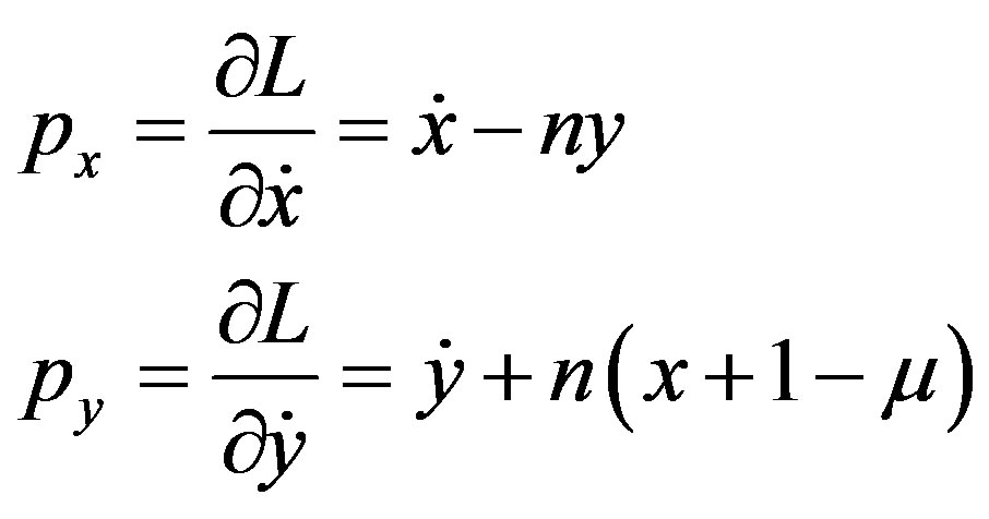
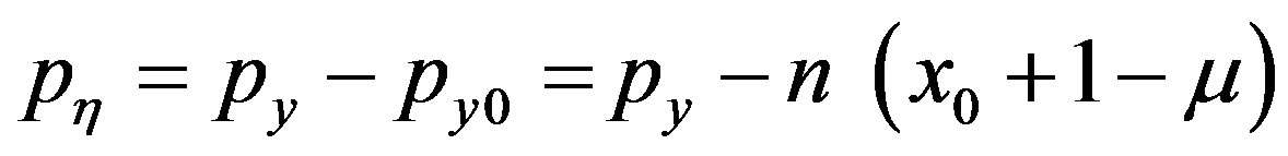
and the canonical variables p_x & p_y for Hamiltonian variables

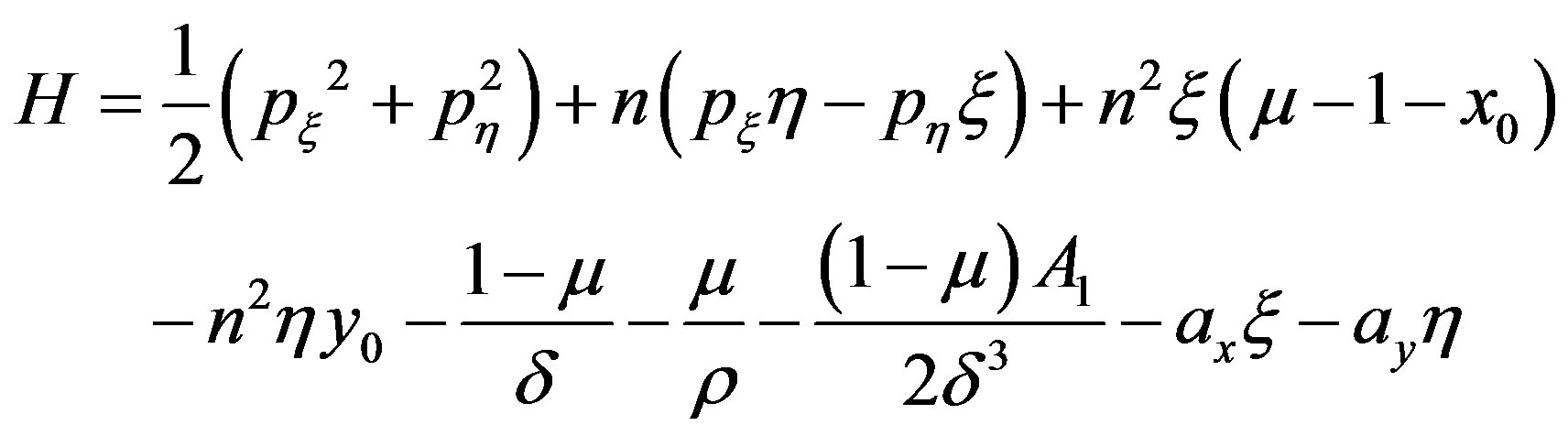
Hence the Hamiltonian H may be written as.

Yielding H as given by

(3.1)

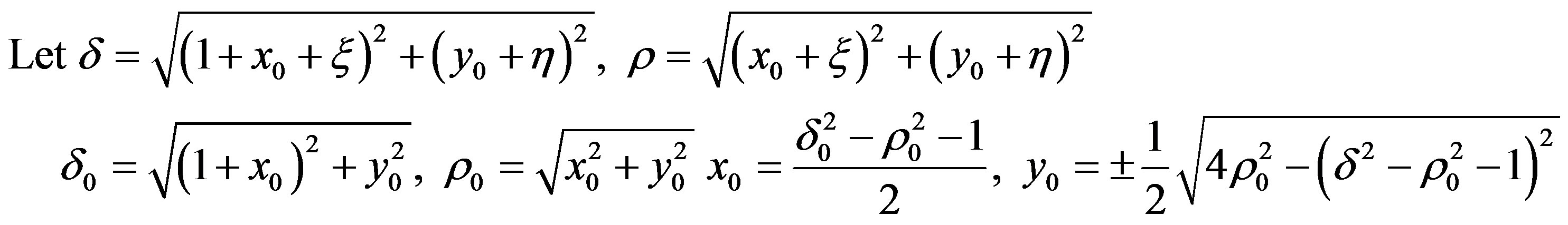
Now let us transfer the origin to the equilibrium point and the new coordinates be written as, so that

Hence the transformed Hamiltonian may be written after eliminating the constant term as

where,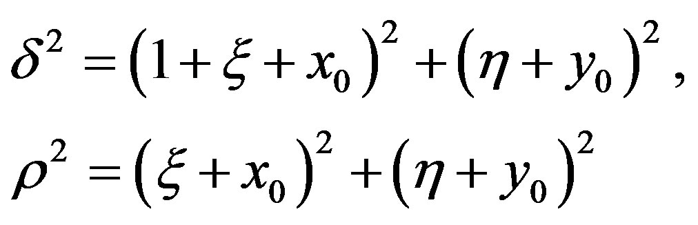

Now expanding H in powers of, we shall have

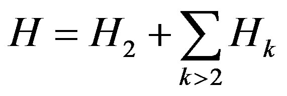
where,

(3.2)

and = functions of, , or, and they are given by (Refer to Appendix Section I(a))

4. Linear Stability Conditions

Hence the Linearized equations of motion may be written as

(4.1)

The corresponding characteristic equation will be

(4.2)

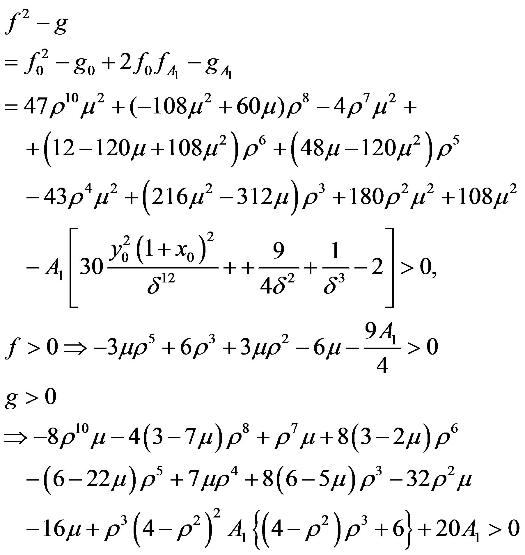
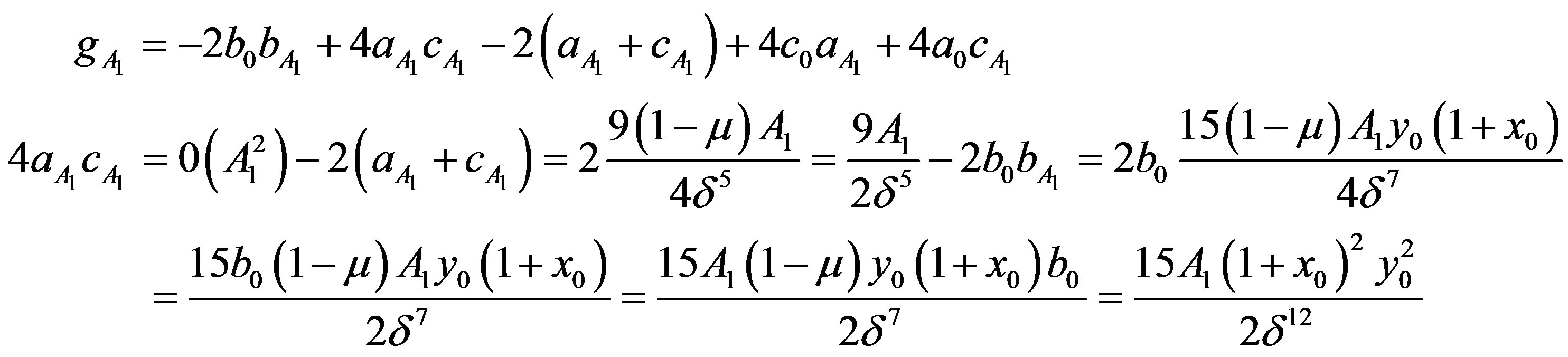
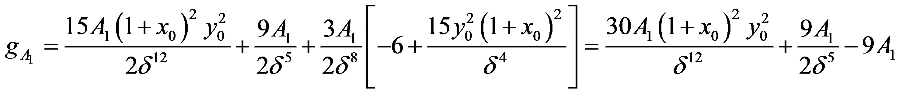
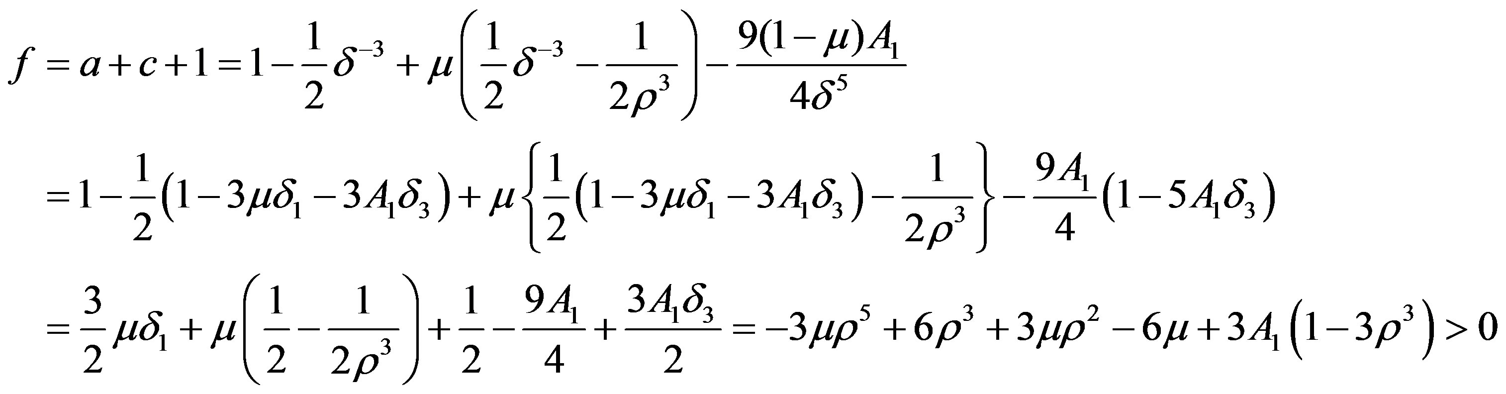
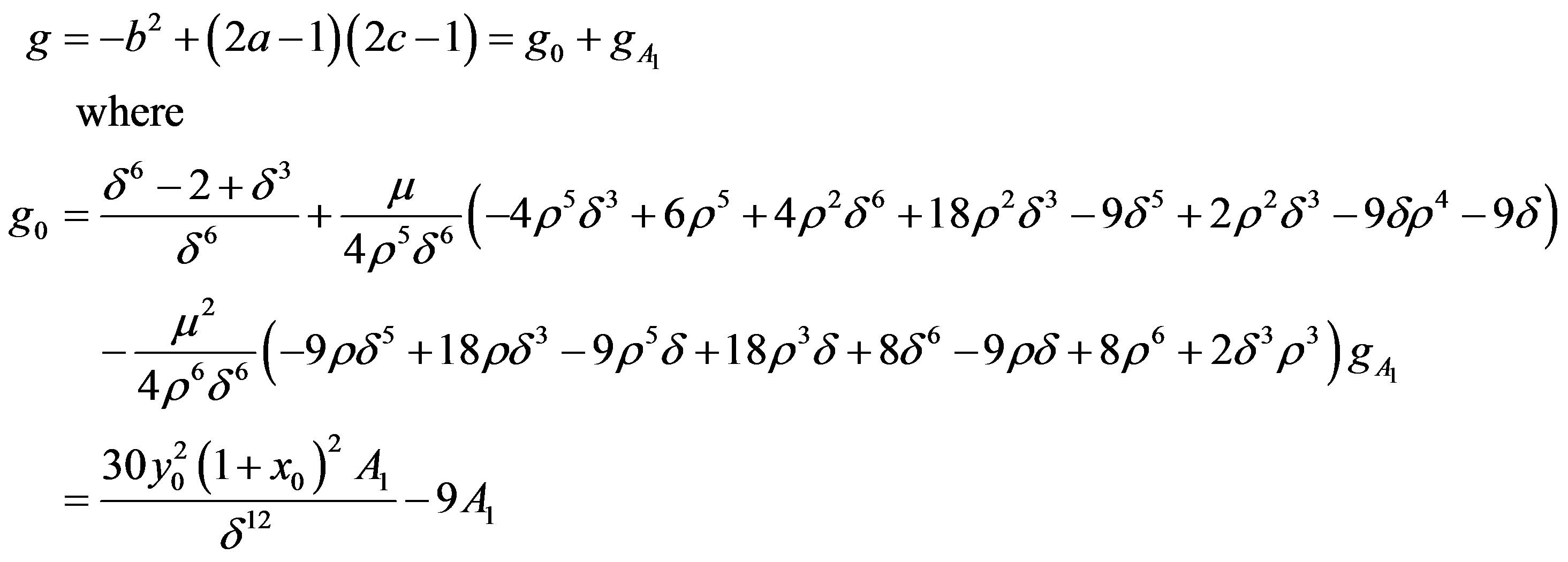
where f and g may be written as

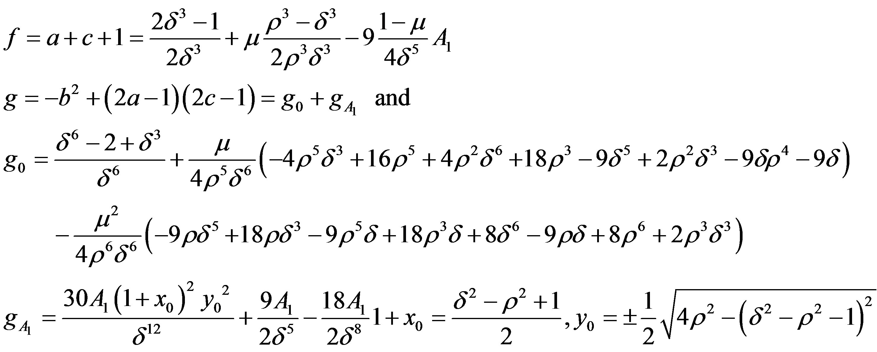
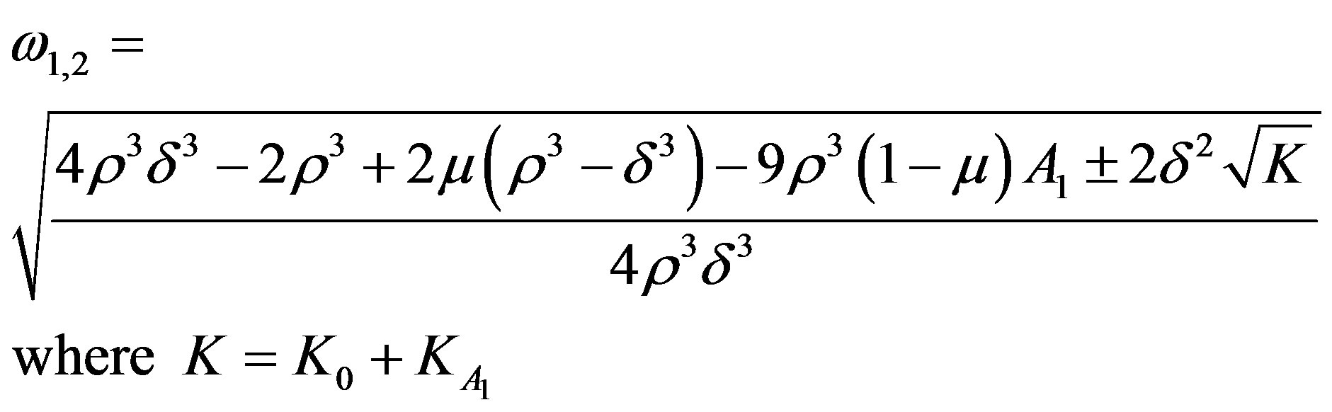
If be the two oscillation frequencies, then they will be given as

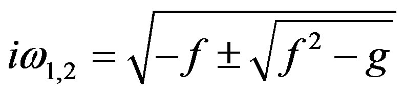
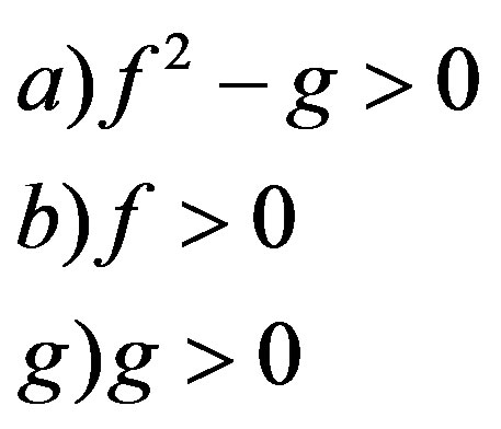
and for linear stability we must have

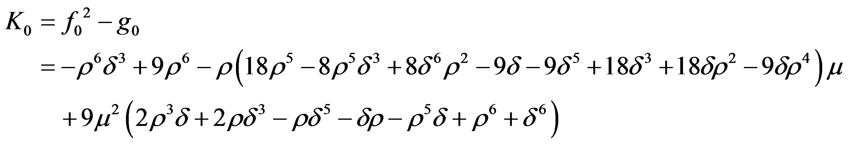
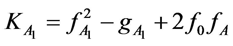
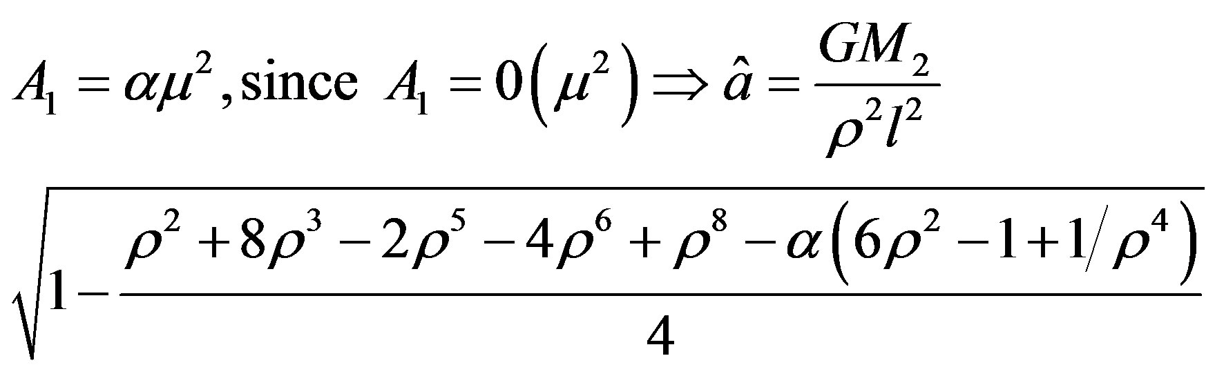
Putting the value for in the expression for, we get

5. Minimum Control Artificial Equilibrium Points

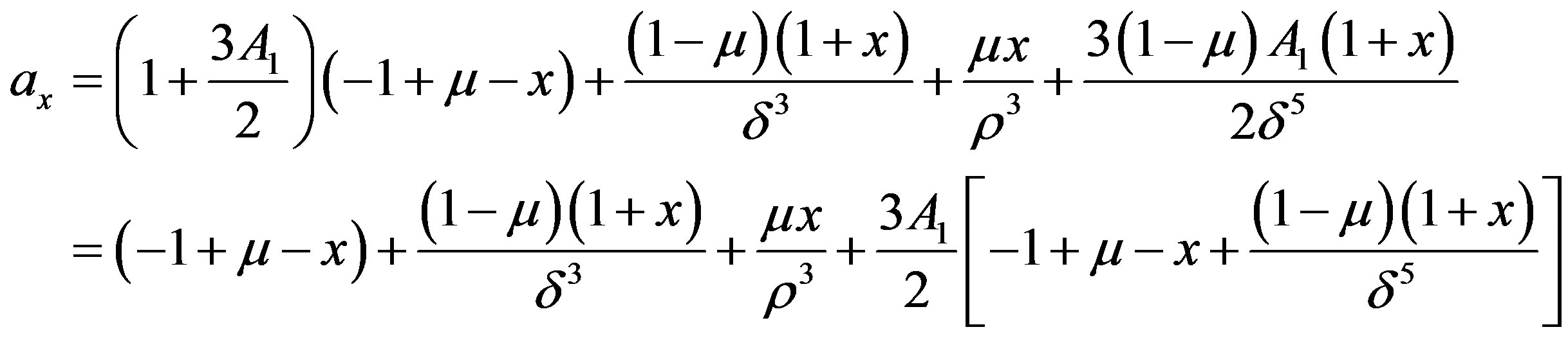
To minimize the objective function, let us consider and writing the value for a_x & a_y, we get

whence we have

Now putting and equating the corresponding coefficients of μ, μ² & A₁ to zero, we get

(5.1)

and the value of corresponding to these δ₀, δ₁, δ₂ & δ₃ will be the maximum value of.

Hence we have,

(5.2)

where, we have taken

will be the corresponding dimensional acceleration, being taken to be the distance between the primaries. It may be verified that when and, the result (5.1) & (5.2) are constant giving the control acceleration to be zero.

Let us look for an analytical estimation of minimum distance from the second primary (ρ) allowing the linear stability conditions. We have

We have ignored the term of the in the expression for and and those in the expression for, hence we get equation for ρ as

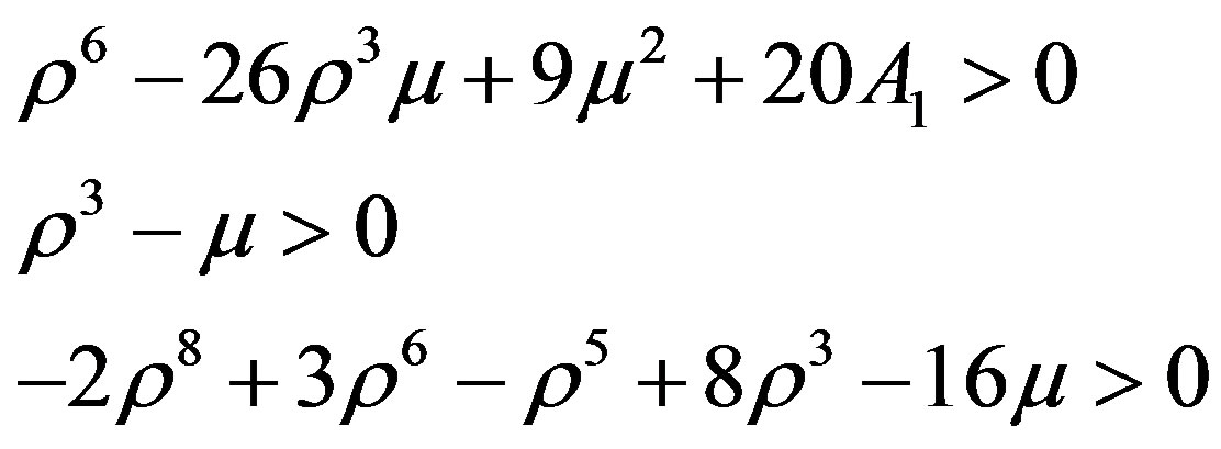
From the 1^st two conditions we obtain our stability boundary limit, i.e.;

[Since]

For earth-moon and

and so it may be checked as.

Thus the value coincides with the value attained by [Bombardelli] and the corresponding control acceleration at the boundary will be

In dimensional units the minimum distance from the second primary in order to have stability will be

and the required dimensional control acceleration will be

.

So it shows that with the presence of obliquity the amount of acceleration decreases and a lesser power of thrust will be needed.

6. Conclusion

We have investigated the properties of minimum control artificial equilibrium points in the planar circular restricted three-body problem while the effect of the oblateness of the bigger primary body is also taken into account. We have found the analytical expressions which characterize their location, control acceleration and stability properties. It is seen that due to the presence of oblateness in the expression all the properties are likely to be affected and the disturbance is more natural since the study of effect of oblateness is quite necessary for exhaustive study of the effect. The specialty of the presence of the oblateness lies in the fact that the amount of acceleration is less and consequently a less power of thrust is required for the mission.

REFERENCES

Appendix I

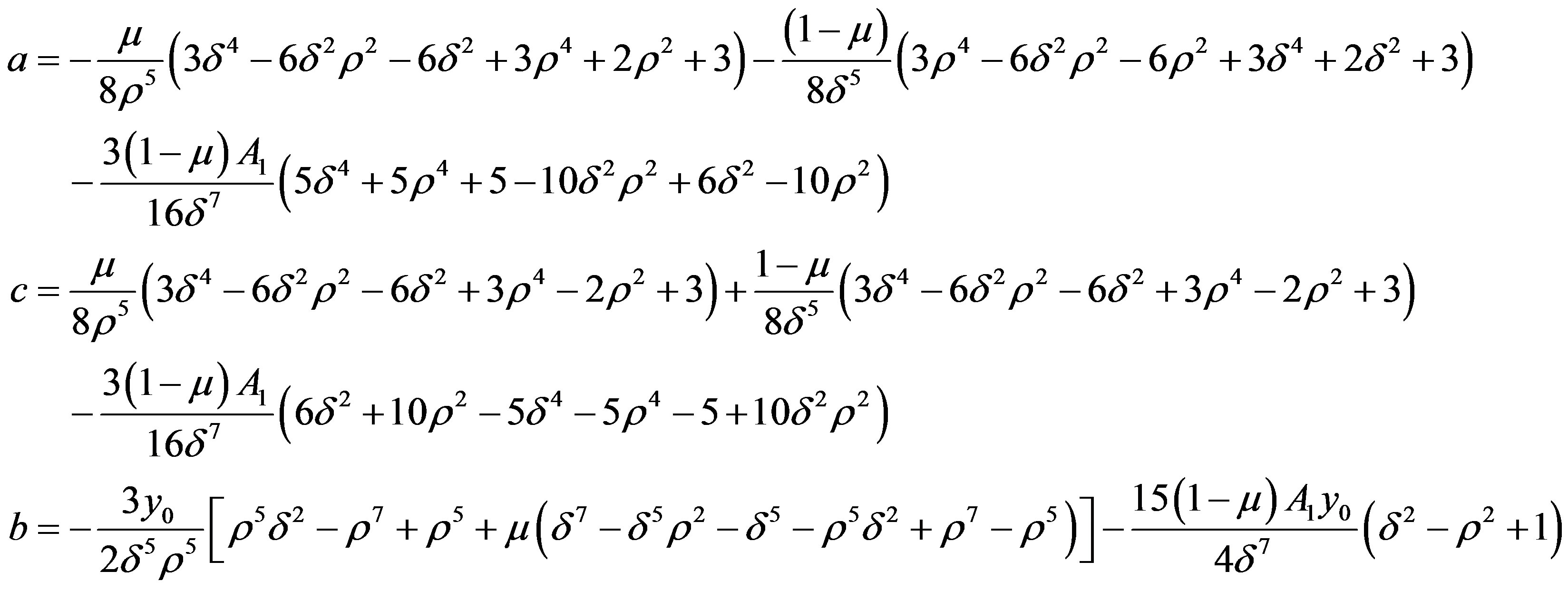
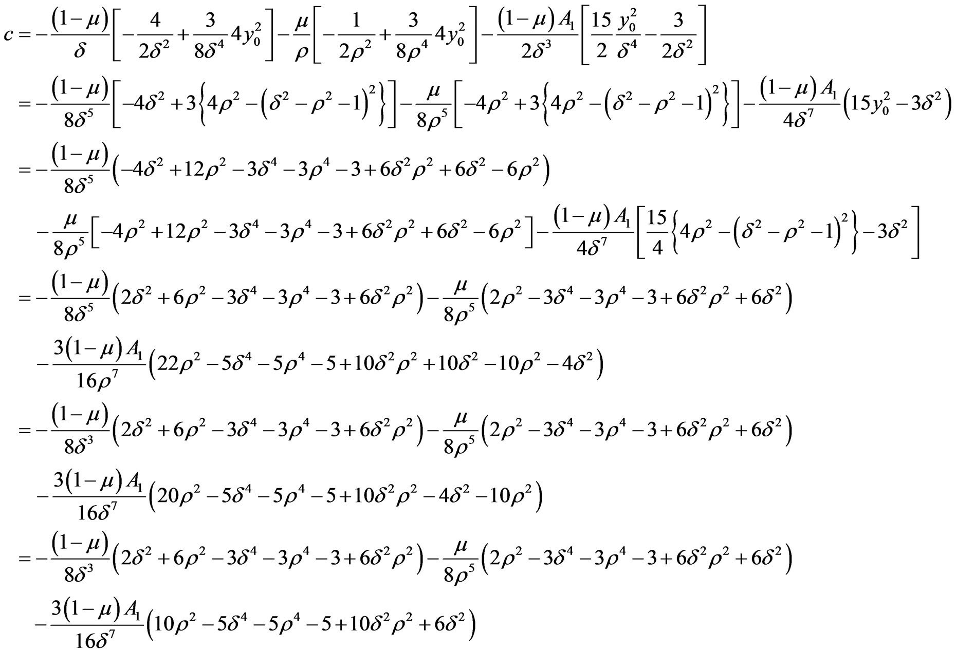
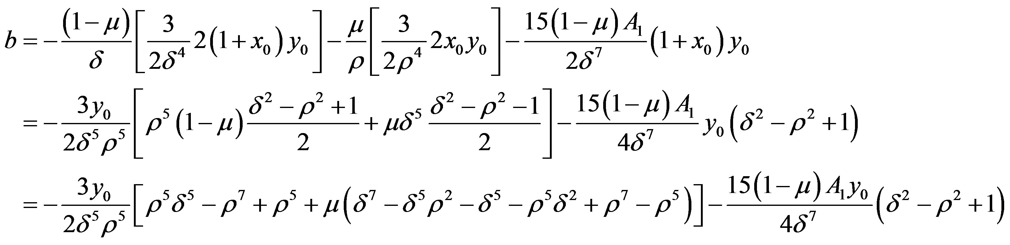
(a) Expression for a, b and c:

Let the suffix (0) denote the terms corresponding to the equilibrium position and the suffix denote the contribution due to the presence of the oblateness of the larger primary body.

Onwards we drop the suffix (0) with.

Now are the coefficients of in the expression for

Appendix II

Expression for and: We shall now onwards ignore second and higher powers of A₁ and also multiple μA₁ and so on. Thus

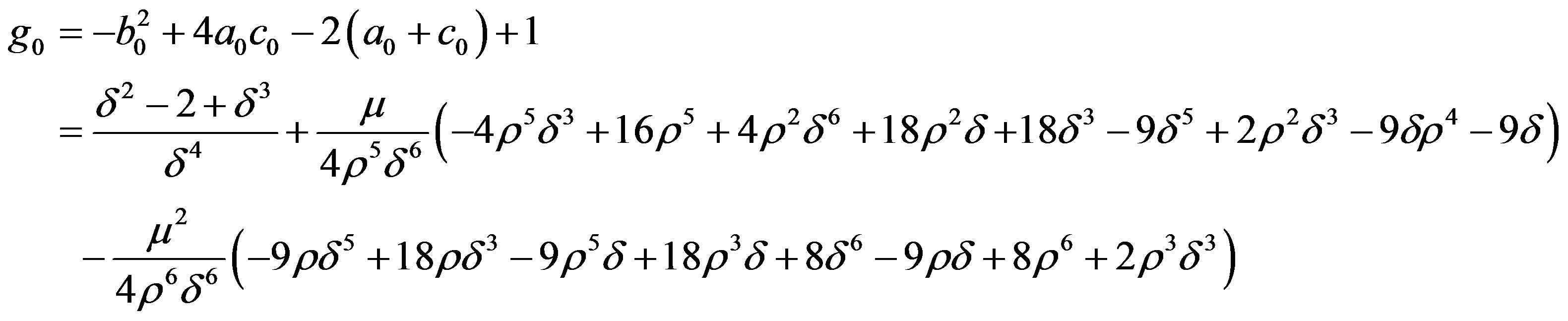
So,

Appendix III

Calculation of

We have

where we have dropped the suffix (0) with x₀, y₀, δ₀, ,

Putting and equating the different corresponding coefficients to zero, we shall get

Appendix IV

Expression for, & for minimum value of δ given by

We shall ignore the terms of the order of and in the expression for but the terms of will be retained in the expression for. thus

Ignoring the terms of the order of and also taking into account, we have

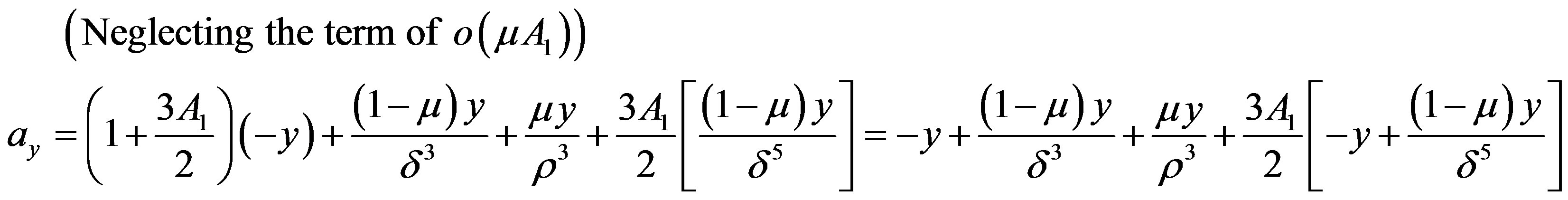
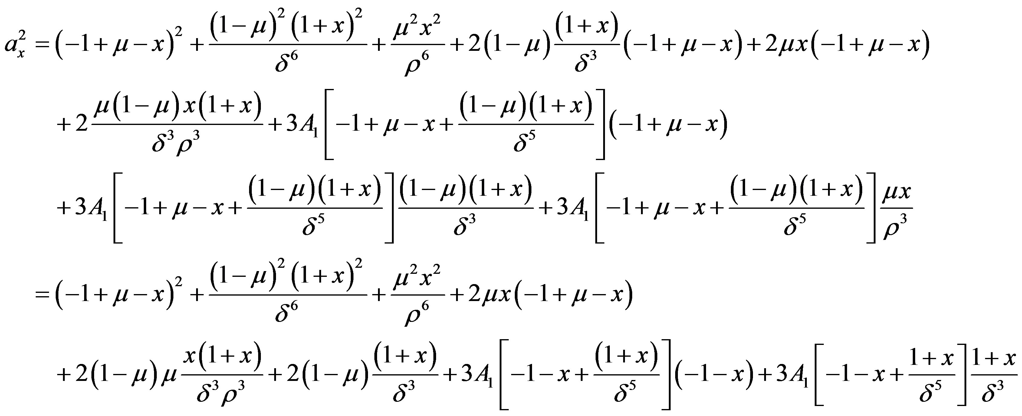
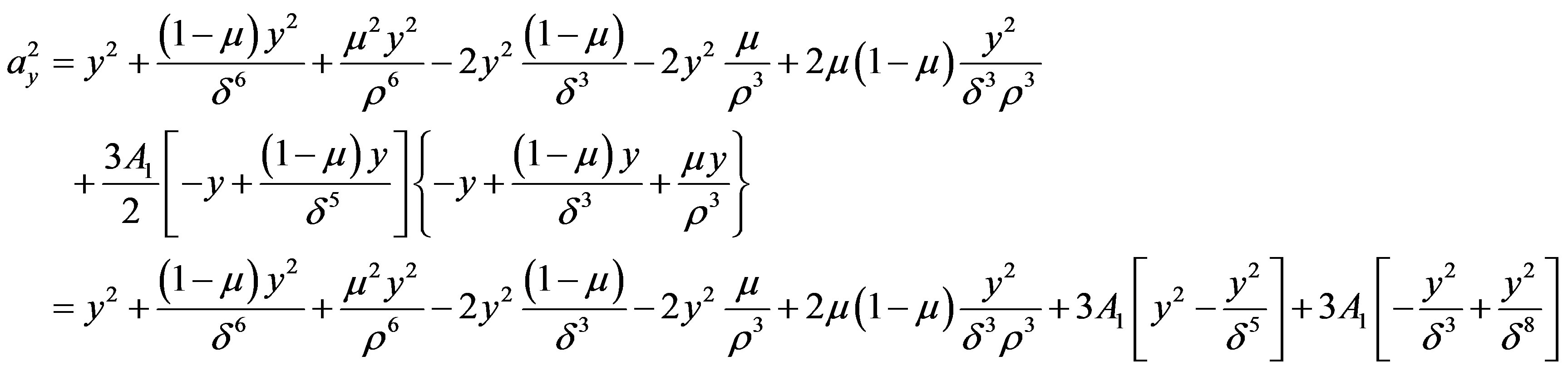
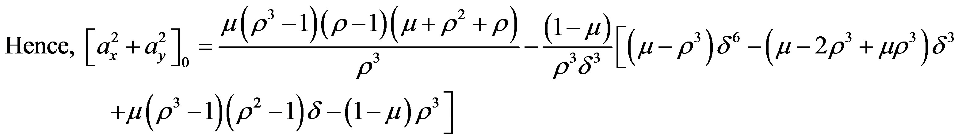
Similarly, we shall have the expression for as follows:

Thus neglecting the terms as mentioned above, we have

REFERENCES

- C. R. Mclnnes, “Solar Sailing Technology, Dynamic and Mission Application,” Springer Application, SpringerPraxis, London, 1999.
- K. E. Tsiolkovsky, “Extension of Man into Outer Space,” In Proc. Symp. Jet Propulsion, Vol. 2, United Scientific and Technical Presses, 1936. (in Russian)
- K. Tsander, “From a Scientific Heritage,” NASA Technical Translation No TTf-541, NASA, Washington DC, 1967.
- R. L. Garwin, “Solar Sailing: A Practical Method of Propulsion within the Solar System,” Jet Propulsion, Vol. 28, No. 123, 1958, pp. 188-190.
- J. L. Wright and J. M. Warmke, “Solar-Sail Mission Applications,” Proceedings of AIAA/AAS Astrodynamics Conference, San Diego, 1976, paper no.AIAA-76-808.
- M. Leipold, “ODISSEE—A Proposal for Demonstration of a Solar Sail in Earth Orbit,” Paper IAA-L98-1005, International Academy of Astronautics, Stockholm, 1998.
- J. M. Logsdon, “Missing Halley’s Comet: The Politics of Big Science,” Isis, Vol. 80, No. 2, 1989, pp. 254-280. http://dx.doi.org/10.1086/355011
- M. McDonald and C. R. Mclnnes, “A Near Linear Road Map for Solar Sailing,” Proceedings of the 55th International Astronautical Congress, Vancouver, 4-8 October 2004.
- A. Markeev, “Stability of the Triangular Lagrangian Solutions of the Restricted Three-Body Problem in the Three Dimensional Circular Case,” Soviet Astronomy, Vol. 15, No. 4, 1972, pp. 682-686.
- C. R. Mclnnes, A. J. C. McDonald, J. F. L. Simmons and E. W. MacDonald, “Solar Sail Parking in Restricted Three Systems,” Journal of Guidance, Control, and Dynamics, Vol. 17, No. 2, 1994, pp. 399-406.
- H. M. Dusek, “Motion in the Vicinity of Libration Points of a Generalized Three Body Model,” AIAA/IODI Astrodynamics Specialist Conference, AIAA, Monterey, 16-17 September 1965, pp. 565-682.
- A. A. Perezhogin, “Stability of the Sixth and Seventh Libration Point with Photo-Gravitational Restricted Circular Three Body Problem,” Sovt. Astron. Zh., 1976, pp. 174-175.
- A. L. Kunitsyn and A. A. Perezhogin, “On the Stability of Triangular Libration Point of the Photo-Gravitational Restricted Problem of Three Bodies,” Celest. Mech. Dyn. Astron., Vol. 18, 1978, pp. 395-408.
- G. Mengali and A. A. Quarta, “Non-Keplerian Orbits for Electric Sails,” Celestial Mechanics and Dynamical Astronomy, Vol. 105, No. 1-3, 2009, pp. 179-195. http://dx.doi.org/10.1007/s10569-009-9200-y
- M. Y. Morimoto, H. Yamakawa and K. Uesugi, “Artificial Equilibrium Points in the Low-Thrust Restricted Three-Body Problem,” Journal of Guidance, Control, and Dynamics, Vol. 30, No. 5, 2007, pp. 1563-1567. http://dx.doi.org/10.2514/1.26771
- R. L. Forward, “Statite: A Spacecraft That Does Not Orbit,” Journal of Spacecraft and Rockets, Vol. 28, No. 5, 1991, pp. 606-611. http://dx.doi.org/10.2514/3.26287
- C. Bombardelli and J. Pelaez, “On the Stability of Artificial Equilibrium Points in the Circular Restricted ThreeBody Problem,” Celestial Mechanics and Dynamical Astronomy, Vol. 109, No. 1, 2011, pp. 13-26. http://dx.doi.org/10.1007/s10569-010-9317-z
- P. V. Subba Rao and R. K. Sharma, “Effect of Oblateness on the Non-Linear Stability of L4 in the Restricted ThreeBody Problem,” Celestial Mechanics and Dynamical Astronomy, Vol. 65, No. 3, 1997, pp. 291-312.
- V. Kumar and R. K. Choudhary, “On the Stability of the Triangular Lagrangian Points Radiating as Well,” Celestial Mechanics and Dynamical Astronomy, Vol. 40, 1987, pp. 155-170.
- S. W. McCusky, “An Introduction to Celestial Mechanics,” Addison-Wesley, New York, 1963.
- V. Szebehely, “Theory of Orbits: The Restricted Problem of Three Bodies,” Academic Press, New York, 1967.
- V. Coverstone and J. E. Prussing, “Technique for Escape from Geosynchronous Transfer Orbit Using a Solar Sail,” Journal of Guidance, Control, and Dynamics, Vol. 26, No. 4, 2003, pp. 628-634. http://dx.doi.org/10.2514/2.5091