Open Journal of Statistics, 2012, 2, 184-187
http://dx.doi.org/10.4236/ojs.2012.22021 Published Online April 2012 (http://www.SciRP.org/journal/ojs)
On a Generalized Model in Accelerated Life Testing
Eduardo L. Cruz1, Adolfo M. De Guzman2
1Department of Epidemiology and Biostatistics, University of the Philippines, Manila, Philippines
2School of Statistics, University of the Philippines, Quezon City, Philippines
Received January 30, 2012; revised February 29, 2012; accepted March 14, 2012
ABSTRACT
The main objective of accelerated life tests in this setting is the recovery of the distribution of the random variable rep-
resenting lifetime which is difficult to observe at a certain level of a given stress factor. A general model for accelerated
life test is proposed that utilizes the inverse prob lem approach, that is, the variable is observ e at different level/s and the
transfer function is used to recover the elusive random variable (life time). The problem then is reduced to finding the
transfer function. We derive some properties of the proposed general model. The Lognormal distribution and the Ar-
rhenius model for lifetime are used as examples. Its relationship with the Cox proportional hazards model is also dis-
cussed.
Keywords: Accelerated Life Test; Arrhenius Model; Inverse Problem
1. Introduction
From the point of view of production and reliability en-
gineers, accelerated life testing is an important aspect of
product development, quality control and improvement.
Accelerated life testing is accomplished by applying in-
creased stress on the product or product component. It is
intended to produce data on strength and on lifetime of
material components and systems. For an excellent but
elementary exposition on this, the reader is referred to
Nelson [1].
Accelerated life testing is also very interesting from
the point of view of theory. Most lifetime data suffer
from the censoring problem of statistics. Lifetime obser-
vations usually exceed the interest time of the observer or
even his own lifetime. Accelerated life tests, however,
are performed to destruction thereby eliminating cen-
sored observations. The analysis of censored or incom-
plete data requires a modification of the usual statistical
methodology of independent and identically distributed
observations and their uncensored generalizations. Re-
cent developments point to the counting process approach
with the use of martingales as introduced by Aalen [2]
for analyzing survival or lifetime data. The audience is
referred to Anderson, Borgen, Gill and Keiding [3] and
Fleming and Harrington [4] for a comprehensive treat-
ment. The first volume covers extensively both theory
and applications of the counting process approach to sur-
vival analysis while the second volu me treats the analysis
of clinical data via the martingale approach. Both books
require some amount of mathematical as well as statisti-
cal sophistication. It takes more time for this approach to
be a practical statistical technology. An alternative to the
counting approach is provided by the Accelerated Life
Testing in some interesting cases. This is so because it
reduces the number of incomplete observations and even
eliminate them.
Section 2 of this paper describes a generalized model
for accelerated life testing. Its properties are stated and
discussed in Section 3 where some examples are also
provided. Section 4 gives some concluding remarks and
future work.
2. A Generalized Model for Accelerated Life
Test
Let X be a nonnegative random variable that represents
lifetime in the normal condition, that is, without any
stress applied to it, with unknown distribution F. Suppose
stress is applied on X and the observations say,
12
X
,,,
s
sns
XX
:S S
are made from a distribution, say Fs.
This setting is an example of the inverse problem ap-
proach in statistics where the stress S is a known operator.
That is,
X
X:S SF F
,,,
or , (1)
in some space of random variables. Here the stress s may
have K levels, i.e. 12
K
s
ss.
An approach to accelerated life test model is given by
Cox and Oakes [5] and Barlow and Sheuer [6] and also
appears in Gnedenko, et al. [7]. This is described as fol-
lows. Denote a failure time distribution function under a
C
opyright © 2012 SciRes. OJS

E. L. CRUZ ET AL. 185
normal stress condition by F0(·). The accelerated life
time transformation is given in terms of


,
F
tz
 
0
,,
and
F0(·) by the relat ionship

F
tzF tzA   


,zA 

,zA
 
,
, (2)
where is a positive function (or acceleration
function) connecting “time to failure” with a stress factor
z, and A is a vector of unknown parameters. For z = 0,
is assumed equal to 1. This relationship is a
scale transformation where a change in stress does not
result in a chang e in the sh ape of the distribution function
but changes its scale only. This relationship can be writ-
ten in terms of the acceleration function as

g
tzAt  . (3)
In other words, the relationship above is linear with a
time acceleration function

.
We now propose a model for accelerated life test gen-
eralizes the relationship in (3). This general model is
expressed in terms of random variables and thus is sim-
pler in structure. Let S be a nonempty set whose elements
we will refer to as stress space. For example, in the Ar-
rhenius model, S is the set of nonnegative real numbers
representing temperature. We define the proposed model
by

,
s
X
As X  

,
, (4)
where X is the random variable under normal use,
 is a
vector of parameters, s  S and
A
s

is called the
scaling or acceleration function which is a monotone
function continuous from the right. This model is a sto-
chastic process S

:

X
sS and will be called a general
lifetime model with stress space S. The model says the
random lifetime S
X
depends on the stress s, where stress
is a state or configuration of stress factors belonging to
some known stress space S. Information on the stress
space should be available in the underlying field such as
medicine for clinical trials, psychology for behavioral
studies, chemistry for phenomena depending on clinical
reactions, to name a few.
Two situations arise from this model: first, if stress s is
fixed or controlled, this model is interpreted as a general
accelerated life test model. If s is random, the model is
known as the survival model with covariates. In this pa-
per we consider only the first case where stress s is fixed.
We will refer to this model as the Generalized Model for
Accelerated Life Testing (GMALT). It will be shown
how this model relates to the well-known Arrhenius
model in reliability engineering. The Arrhenius model is
widely used to model product life as a function of tem-
perature. Applications include electrical insulations, solid
state and semiconductor devices, battery cells, and in-
candescent lamp filaments.
3. Elementary Properties of the GMALT
and Some Examples
As mentioned in the introduction, the main advantage of
the proposed model which is expressed as a scaling of
random variables is that its properties can be studied
more conveniently. In this section we present some ana-
lytic properties of the proposed model and state them as
propositions.
3.1. Mean and Covariance Function
Proposition 1. If S
X
is a gmalt with acceleration func-
tion


,
A
s

and stress space S, then the mean function
μs and the covariance function

2,
s
t
 are given by,








,,
X
sAsEX As

 
s
, S

 
and




2,
2
,, ,
,,,
XX st
X
EAs XAsAt
As At









20
 


2
22
,X
SAs
where μX and X are the mean and variance of the
untransformed X, respectively. In particular, the variance
at any stress s  S is

 

. The proof of
these is straightforward and follows from the properties
of expectation. To keep things simple, we write A(s) in-
stead of


,
A
s

from now on.
The next property shows the effect of log transforma-
tion in the GMALT model. The proof follows directly
from applying the definition of logarithmic function and
mathematical expectation.
3.2. Effect of Log Transformation


glo S

S
Proposition 2. If
X
As X, then
X
has
constant variance

2Var logS
X
  and mean


0log
given by
 


, (6)


log
where 0
A
s  



log
So the log transformation results in a constant variance
but a changing mean. In particular, since
and .

logEX  




0, 1As

log 0As ,
the mean decreases since . An interesting
case is when


log
X
S has a Normal distribution.
Example 1. (Lognormal model) In the GMALT, S
X
is
Lognormal with mean S

2 and variance S

log if
s
X
is normal with mean, say

2 and variance


S
. In this
case the parameters of

2
exp 2
Sb
 

X
are and




22 22
expexp 1
Sb






expb



where

, and

2 and

 are as defined in Property 2 (See Hogg and
Craig [8] for pr operties of Lognormal distribution).
This example will enable us to make inferences about
X which is not observed in the GMALT model via the ac-
celeration function A(s), when it is known.
In the next example we show a situation where the

E. L. CRUZ ET AL.
186
model in Equation (4) fails. This example is also used to
verify the second property which states the effect of log
transforma tion on the GMALT.
Example 2. The data in Table 1 are hours to turn fail-
ure of a new Class-H insulation system tested in Motor-
ettes at 190, 220, 240, and 260 Temperature (˚C). The
original purpose of the experiment was to estimate the
median time to turn failure at the design of 180 Tem-
perature (˚C) [1].
To verify the second property in Section 3.2, we com-
pare the variances of the untransformed and the log-
transformed gmalt model. But we will see that Property 2
is satisfied on the three temperature levels only, as the
stress level 260 Temperature (˚C) seemed to have violat ed
an assumption of accelerated life model. In Tables 2 and
3 we see that the variances of both the untransformed and
the log-transformed lifetime at all temperature levels are
statistically different, but is not so for the first three lev-
els, where the variances of the log-transformed data are
not statistically different. Our observation, is that failure
Table 1. Hours to failure in an accelerated life test of class H
insulation in Motorettes.
Temperature (˚C) Levels
190˚C 220˚C 240˚C 260˚C
7228 1764 1175 600
7228 2436 1175 744
7228 2436 1521 744
8448 2436 1569 744
9167 2436 1617 912
9167 2436 1665 1128
9167 3108 1665 1320
9167 3108 1713 1464
10511 3108 1761 1608
10511 3108 1953 1896
Table 2. Test of homogenity of variance (all temperature
levels) of hours to failure and its log transformation Motor-
ettes data.
Life time of Motorette Levene Statistic Significance
Hours to failure 9.962 0.000
Log (Hours to failure) 8.373 0.000
Table 3. Test of homogenity of variance (190, 220 and 240
Temperature (˚C) levels only) of hours to failure and its log
transformation in class H insulation in Motorettes data.
Life time of Motorette Levene Statistic Significance
Hours to failure 7.708 0.001
Log (Hours to failure) 0.712 0.553
modes are different at these two sets of levels (the 190,
220 and 240 Temperature (˚C) degrees, and the 260
Temperature (˚C)), and that the stress level 260 Tem-
perature (˚C) may have destroyed the shape of the distri-
bution, thus violating the scaling assumption of the mo d e l ,
where a change in stress does not result in a change in
the shape of the distribution function but changes its
scale only. So, in this example we see that for the first
three temperature levels, the log transformation has re-
sulted in a constant variance but with still different (de-
creasing) mean, thus verifying Property 2. For this ex-
ample, therefore th e proposed model is applicable on the
first three stress levels only. The following will be useful
in interpreting the log mean of S and X.
X
Proposition 3. If Z is a log symmetric random variable
with log mean S



, i.e.


logEZ S

, then




exp median
Z
S
 
, where S

 is as in Example 1.
Proof of Propositio n 3. From symmetry we have




log1 2
S
PZ  
.
Since





log exp
SS
PZ PZ  






 
exp median
S
F
FZ 

then





, where F is the
distribution fun c tion of Z.
The result follows for absolutely continuous distribu-
tion functions F. We next relate the mean


2 and vari-
ance

 to the mean and variance of the untransformed
or “normal use” random variable X. To do that we need
the next result.
Proposition 4. Let X be a any nonnegative random
variable with distribution function F and finite mean


EX  

2
EX
2
F and second moment . Then there
exists positive numbers
F

and
F

such that,


logEX and . In

F



2
22
Var logFFF X   

1
d
F
x
Fx 



22
0
d
y
F
and
x
fact, Fx  
logyx
where
. We may now state the next property.


Proposition 5. In the GMALT model with accelera-
tion function




0, 1As
S
and stress space S, the ex-
pectations and variance of the log transformation of
X
have the properties



log log
SFF
EX As



, (8)
and


2
Var logSFF X

 
2
, (9)
where the random variable X with distribution F satisfies
the usual regularity conditions and
F

and
F

, are as
in Proposition 4.
The next result states the equivalence of our approach
to the classical Arrhenius model where the acceleration
function is given by

E. L. CRUZ ET AL.
187
 
12
exp
A
ss  

0,s
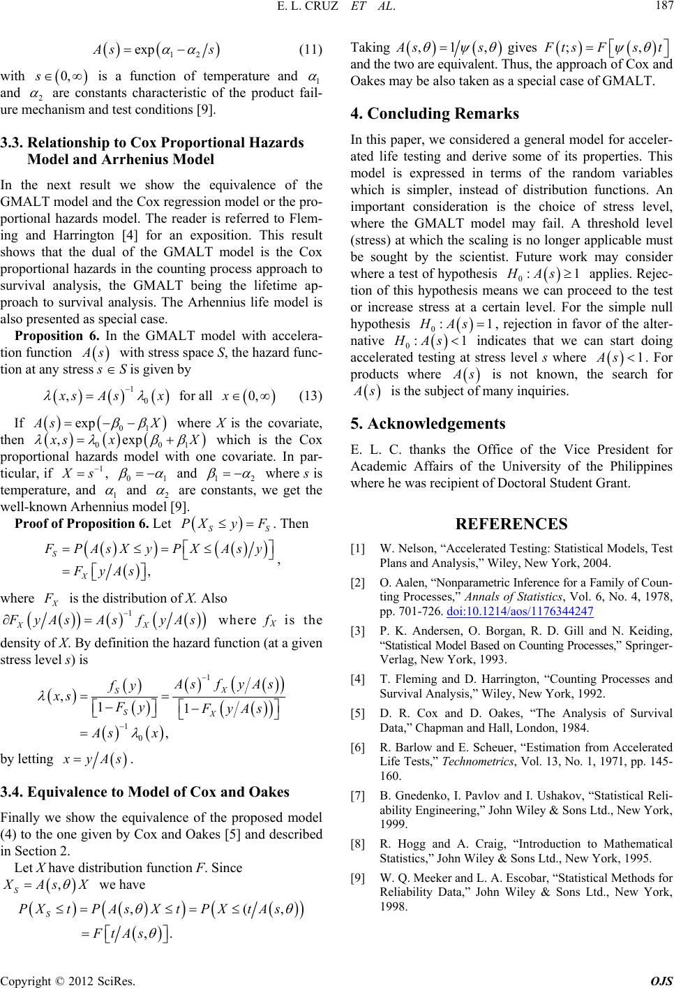
(11)
with is a function of temperature and 1

and 2

are constants characteristic of the product fail-
ure mechanism and test conditions [9 ].
3.3. Relationship to Cox Proportional Hazards
Model and Arrhenius Model
In the next result we show the equivalence of the
GMALT model and the Cox regression model or the pro-
portional hazards model. The reader is referred to Flem-
ing and Harrington [4] for an exposition. This result
shows that the dual of the GMALT model is the Cox
proportional hazards in the counting process approach to
survival analysis, the GMALT being the lifetime ap-
proach to survival analysis. The Arhennius life model is
also presented as special case.
Proposition 6. In the GMALT model with accelera-
tion function

A
s

1
with stress space S, the hazard func-
tion at any stress s  S is given by

,

0
x
sAs


0,x

01
x   for all (13)
If

exp
A
sX  

xp
where X is the covariate,
then 01
 
0
,e
x
sx
1
X    which is the Cox
proportional hazards model with one covariate. In par-
ticular, if
X
s, 01

  and 12

  where s is
temperature, and 1

and 2

are constants, we get the
well-known Arhennius model [9].
Proof of Propositio n 6. Let . Then

SS
PXy F









,
S
X
F
PAsX yPX
FyAs



As y



,
where X
F
is the distribution of X. Also
    
X
1
X
F
yAs As

fyAs where fX is the
density of X. By definition the hazard function (at a given
stress level s) is
 

 

 
 
1
1
0
,11
,
S
SX
X
A
sfyAs
FyAs



fy
xs Fy
As x









by letting
x
yAs

,
.
3.4. Equivalence to Model of Cox and Oakes
Finally we show the equivalence of the proposed model
(4) to the one given by Cox and Oakes [5] and described
in Section 2.
Let X have distribution function F. Since
S
X
As X   we have
  

 

, .
S
PXtPAsX tPX
FtAs
,(
,tAs

 







Taking




,1,
A
ss  



;,
F
tsFs t   gives





and the two are equivalent. Thus, the approach of Cox and
Oakes may be also taken as a special case of GMALT.
4. Concluding Remarks
In this paper, we considered a general model for acceler-
ated life testing and derive some of its properties. This
model is expressed in terms of the random variables
which is simpler, instead of distribution functions. An
important consideration is the choice of stress level,
where the GMALT model may fail. A threshold level
(stress) at which the scaling is no longer applicable must
be sought by the scientist. Future work may consider
where a test of hypothesis 0 applies. Rejec-
tion of this hypothesis means we can proceed to the test
or increase stress at a certain level. For the simple null
hypothesis

:1HAs


0:1HAs

, rejection in favor of the alter-
native


:1HAs
0

indicates that we can start doing
accelerated testing at stress level s where

1As

. For
products where


A
s is not known, the search for


A
s is the subject of many inquiries.
5. Acknowledgements
E. L. C. thanks the Office of the Vice President for
Academic Affairs of the University of the Philippines
where he was recipient of Doctoral Stude nt Grant.
REFERENCES
[1] W. Nelson, “Accelerated Testing: Statistical Models, Test
Plans and Analysis,” Wiley, New York, 2004.
[2] O. Aalen, “Nonparametric Inference for a Family of Coun-
ting Processes,” Annals of Statistics, Vol. 6, No. 4, 1978,
pp. 701-726. doi:10.1214/aos/1176344247
[3] P. K. Andersen, O. Borgan, R. D. Gill and N. Keiding,
“Statistical Model Based on Coun ting Processes,” Sp ri ng e r-
Verlag, New York, 1993.
[4] T. Fleming and D. Harrington, “Counting Processes and
Survival Analysis,” Wiley, New York, 1992.
[5] D. R. Cox and D. Oakes, “The Analysis of Survival
Data,” Chapman and Hall, London, 1984.
[6] R. Barlow and E. Scheuer, “Estimation from Accelerated
Life Tests,” Technometrics, Vol. 13, No. 1, 1971, pp. 145-
160.
[7] B. Gnedenko, I. Pavlov and I. Ushakov, “Statistical Reli-
ability Engineering,” John Wiley & Sons Ltd., New York,
1999.
[8] R. Hogg and A. Craig, “Introduction to Mathematical
Statistics,” John Wiley & Sons Ltd., New York, 1995.
[9] W. Q. Meeker and L. A. Escobar, “Statistical Methods for
Reliability Data,” John Wiley & Sons Ltd., New York,
1998.