Journal of Modern Physics
Vol. 2 No. 9 (2011) , Article ID: 7147 , 10 pages DOI:10.4236/jmp.2011.29126
Experimental Investigation of Evolution Process of Nonlinear Characteristics from Chatter Free to Chatter
Department of Industrial Engineering, Jilin University, Changchun, China
E-mail: Kongfs@jlu.edu.cn
Received November 23, 2011; revised April 5, 2011; accepted April 22, 2011
Keywords: Chatter, Uncertainty, Reconstructed Attractor, Lyapunov Exponent and Kolmogorov Entropy
ABSTRACT
The vibration acceleration time history of the cutter holder was separated into three parts; namely, chatter free, transition and chatter processes. The reconstructed attractor and probability distribution of vibration acceleration time series were studied in order to observe the system’s behavior. The Lyapunov exponent andKolmogorov entropy were used to help judge the cutting state. Meanwhile, the relation curves of the Lyapunov exponent and entropy versus machining parameters were plotted and discussed. The research shows that Lyapunov exponent and Kolmogorov entropy are toned up when vibration acceleration time history goes from chatter free, transition to chatter. When cutting state transited from chatter free to chatter, the Lyapunov exponent and Kolmogorov entropy increase with increasing amplitude. In addition, the relation curves looks like stability lobes. The experimental study allow us to select optimal machining parameters for decreasing the uncertainty of cutting vibration.
1. Introduction
Machine tool chatter is the self-excited relative oscillation between the cutting tool and the workpiece developed under large metal removal rates. It deteriorates the workpiece surface, reduces tool and machine life, and may create dangerous accidents. Over the last hundred years, research on this problem have produced many analytical theories. Among these theories, regenerative chatter and mode coupling were identified as the principle theories by Tobias [1] and Tlusty [2]. Merritt [3] presented an elegant stability theory for orthogonal turning using system theory terminology. His formulation was latter adopted by many investigators and led to major advances towards the understanding and prediction of the chatter phenomenon. Hanna [4], Shi and Tobias [5], Tlusty [6] and others carried out theoretical and experimental researches on cutting chatter, explained the mechanism of stabilization of chatter amplitudes and the phenomenon of finite amplitude instability, and presented a non-linear theory of machine tool chatter. Chaos cutting is an important phenomenon which is related to the non-linear theory of machine tool chatter. Grabec [7-9] analyzed the dynamics of cutting and con-cluded that the process was chaotic for a large enough cutting force. Gans [10] conducted an extended analysis of the cutting model analyzed by Grabec, and modified the method to calculate the Lyapunov exponents using sharply varying continuous functions to replace the discontinuities nonlinear dynamical system. Gradisek [11] applied bifurcation diagrams to illustrate the influence of cutting depth on the development of irregular tool oscillations based on Grabec’s model. In another paper [12], Gradisek indicated that at least two cutting regimes from time series cutting forces should be distinguished between chatter-free and cutting accompanied by chatter. The chatter-free cutting regime was described as a linearly correlated random process with weak periodic oscillations; whereas the chatter regime was described as a low dimensional possibly chaotic process with expressive, nearly harmonic oscillations. Satishmohan and Akhlesh [13] found that turning operations exhibit low-dimensional chaos from the surrogate-data test, quasiperiodicity test and Lyapunov exponent test. The concept of the state of a system is powerful even for nondeterministic systems. There is very little research on uncertainty of cutting state when the cutting system proceeds from chatter free to chatter, especially for irregular chatter. In this paper, the dynamic trait of the vibration acceleration time series evolution was studied in detail based on experiments during the transition from chatter free to chatter.
2. Theoretical Foundation of Experiment Research
2.1. Time Delay
The dynamics of machining systems are very complex due to the variety of nonlinear phenomena involved.
It is well-known that models with constant time delay capture the main character of regenerative dynamics and can be used to describe linear stability properties in good agreement with experiments. However, some phenomena can only be explained using more sophisticated models that incorporate varying time delay as well. In the past century, scholars from all over the world have developed a lot of nonlinear analytical models to describe and explain the fundamental properties of the process. Typical of the single-DOF models on which bifurcation studies have been proposed by Hanna & Tobias [4].
 (1)
(1)
where  is the natural frequency of the system,
  is the damping coefficient of the system,
  is the feeding speed index of cutting tools,
  is the dynamic cutting force coefficients,
  is the time delay, which means a period of one revolution,
  is the nonlinear dynamic term, and
 (2)
(2)
where,  , (i = 2, 3) is the nonlinear coefficient. where
  denotes the delayed value of
 .
.
Since the tool experiences vibrations in the y direction as well, the time delay  is not equal to the rotation period
  of the workpiece, but it is determined implicitly by [14]
 (3)
(3)
Here Ω is the spindle speed given in [rad/s] and R is the radius of the workpiece. Thus, the regenerative delay is a state-dependent delay since it depends on the state, both current ( ) and delayed (
 ).
).
Based on the above model, we can use time series of cutting tool vibration experimental data which obtained from the experiment to reconstruct  dimensions of state space
  to investtigate the dynamic characteristics of evolution process of cutting vibration.
2.2. Attractor and Chaos
The space defined by the independent coordinates require to describe a motion is called a state space. For a given system of equation, the coordinates of the state space are well defined. Considering a set of initial conditions, the time evolution of the system will describe trajectories in the state space. These trajectories can be divergent or convergent to a final state generall called attractor. In other words, an attractor is something that “attracts” initial conditions from a region around it once transients have died out. More precisely, an attractor in a subspace A of the state space S with the property that there is a neighborhood of A such that, for every initial condition, the limit of the orbit as time goes to infinity is A. Thus, almost every trajectory in this neighborhood of A passes close to every point of A. Simple attractors can be: point (a system in equilibrium), periodic, quasiperiodic or strange. The strange attractors are divided into two kinds: chaotic and nonchaotic. The chaotic evolution is associated with an attractor with the property that the system decays to a final state, but this state is not periodic and is extremely complex.
2.3. Lyapunov Exponents
Lyapunov exponents provide a measure of the sensitivity of the system to its initial conditions. They exhibit the rate of divergence or convergence of the nearby trajectories from each other in state space and are used to distingguish the chaotic and nonchaotic (periodic or quasiperiodic) behaviors. Periodic attractors show only negative and zero exponents which indicate convergence to a predictable motion, whereas there exists at least one positive exponent for a chaotic system. A positive exponent demonstrates that a pair of very close trajectories diverge as the times evolve. Therefore, one needs to determine the sign of the Lyapunov exponentts to characterize the behavior of a dynamical system.
The definition of the Lyapunov exponents given by Wolf et al. [15] is the following: considering a continuous dynamically system in D-dimensional state space, one monitors the long-term evolution of an infinitesimal D-sphere of initial conditions. The sphere will become a D-ellipsoid due to the local deformed nature of the flow. The ith one-dimensional Lyapunov exponent is defined in terms of the length of the ellipsoidal principal axis 
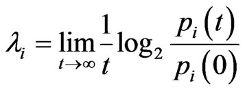
where  are ordered from largest to smaller. The magnitudes of the Lyapunov exponents quantify dynamics in information theoretic terms. The exponent measures the rate at which system processes create or destroy information. Thus, the exponents are expressed in bits of information per second.
2.4. Kolmogorov Entropy
The Kolmogorov entropy (K) is the rate of information loss per unit time (bits per second), and is the sum of the positive Lyapunov exponents. Positive, finite K is generally viewed as a clear indication that the process manifests chaotic dynamics. Very large entropy indicates a stochastic (totally unpredictable) phenomenon. K is estimated from the average number of time steps,  , for two Phase-space points, initially within
 , to diverge to
 . We use the maximum-likelihood form of Grassberger et al. [16].
 , with
  for M point pairs. The data-sampling rate is
 .
.
3. Experiment
3.1. Experimental Setup and Condition
Experiments were conducted on a CA6140 horizontal lathe (as shown in Figure 1) with a cutting speed of 500 r/min, a feed rate of 0.08 mm/r and a cutting depth of 0.6 mm. No coolants or lubricants were used. All the cutting parameters were kept constant during the cutting process. The workpiece was made of steel CS45 (ISO) with a nominal length of 600 mm and a nominal diameter of 50 mm. An accelerometer was attached to a non-standard tool holder with a type SMC cutting insert YT15 and was always perpendicular to the axial line orientation of the workpiece. The overhanging length of the tool holder is 30 mm.
3.2. Experimental Data and Processing
As shown in Figure 2, the vibration acceleration time history was taken from the cutter holder. The experimental analysis shows that it is better to take 5120 Hz sampling rate for the subsequent analysis. The vibration acceleration time history was separated into three parts that were chatter free, transition, and chatter processes based on experiment. The data set applied for estimating the optimum number of embedding dimensions and the data number for computing the Lyapunov exponents is taken from chatter phase and processed with a 8th-order Butterworth band pass digital filter with cut off frequency (60,500) Hz, because we know that the natural frequency of the cutting system is 350 Hz by modal


1-workpiece, 2-turnning cutter, 3-accelerometer, 4-amplifier, 5-oscillograph, 6-AD converter and PC
Figure 1. Schematic diagram of the experimental set-up.
 (a)
(a) (b)
(b)
Figure 2. Diagram of the time history of chatter evolution. Spindle speed 500 r/min, feed speed 0.08 mm/r, cutting depth 0.6 mm. (1) Chatter free phase, (2) Transition phase, (3) Chatter phase.
analysis.
3.3. Selection of Embedding Dimension and Data Number
As we know that, it is important to select the suitable embedding dimension and data number for estimation of Lyapunov exponents by using Rostentein’s method [17]. The computing time of the Lyapunov exponents will be doubled when the embedding dimension increases by one. So it is necessary to optimize the number of embedding dimensions for computing the Lyapunov exponents. With experiment and calculation analysis we find that the Lyapunov exponent will keep constant when the embedding dimension is greater than 5 as shown in Figure 3.
Therefore, we take the embedding dimension equal to five in the following analysis. In view of theory, the greater the data number the better the analysis result, but the computing time will become longer. The problem that needed to be solved is to find the smallest data number the ensures satisfactory analysis result. The research shows that the fluctuation of the Lyapunov exponent against data number is small as the number of data is more than two thousand and five hundred as shown in Figure 4. Therefore, we take the number of data to be equal to two thousand and five hundred in the following analysis.
4. Experimental Analysis of Uncertainty of Evolution Process on Time Series from Chatter Free to Chatter
As shown in Figure 2, the vibration acceleration time history from the cutter holder was separated into three parts; namely, chatter free, transition and chatter processes based on experiment. But the time series analysis methods applied here to analyze these segments require data to be taken from stationary processes. As defined above, the transition segment cannot fulfill this assumption. So we will discuss the uncertainty of evolution process on time series from chatter free to chatter based on two parts, chatter free and chatter segment as shown in Figure 2. A large class of systems can be described by a set of states and some kind of transition rules which specify how the system may proceed from one state to the other [18]. If a nonlinear dynamical system is in a chaotic state, prediction of the time history of the motion is impossible because small uncertainties in the initial conditions lead to divergent orbits in the phase space. If damping is present, we know that the chaotic orbit lies somewhere on the strange attractor. Failing specific knowledge about the whereabouts of the orbit, there is increasing interest in knowing the probability of finding the orbit somewhere on the attractor. One suggestion is to find a probability density in phase space to provide a statistical measure of the chaotic dynamics [19,20]. We now begin by examining the trajectories in the threedimensional reconstructed phase space (x(t), x(t + delay), x(t + 2 delay)), as shown in Figure 5, where the delay equals to 3 (
( equals to 1/5120). The first case is random, since the trajectory continues to be in place as shown in Figure 5(a). The situation in Figure 5(b) is more complicated. Although it is difficult to tell exactly what has happened from this diagram, it looks like it is in a week chaotic state the reconstructed attractors becomes stretched and folded. Secondly, we observed the probability density distribution for two stages of cutting vibration corresponding to Figure 2(c). The distributions have been projected onto the position axis as shown in Figure 6.
The distribution of the first stage shows a shape similar

Figure 3. Sketch of Lyapunov exponent versus embedding dimension with 3000 datum.

Figure 4. Sketch of Lyapunov exponent versus data number here embedding dimension m = 5.
 (a)
(a) (b)
(b)
Figure 6. Probability density distribution of time series for chatter free and chatter corresponding to Figure 2(c).
to a bell shaped curve (Figure 6, curve-a). This distribution is similar to that of a stability vibration. The amplitudes of displacements are smaller and most of them are near zero. In the second stage, the distribution of displacements shows a shape similar to a Gaussian bell shaped curve, but with a fluctuating curve at the top (Figure 6, curve-b). It suggests that the amplitudes of displacements would begin to show diversity. And the displacement of cutting vibration distributes in a wide range. It is difficult to predict the state of cutting vibration. We can deduce that the cutting vibration is of a chaotic characteristic. Reconstructed attractors and probability density distribution of the amplitude of displacements, when they can be obtained, can often provide graphical evidence for nonlinear behavior, such as chaos. However, quantitative measures of nonlinear dynamics are also important. We now discuss the property of evolution of Lyapunov exponents and Kolmogorov entropy with time. As it is known, the Lyapunov exponents are the average exponential rates of divergence or convergence of nearby orbits in phase space and they may be used to obtain a measure of the sensitive dependence upon initial conditions that is characteristic of chaotic behavior [21]. The entropy may be interpreted as a measure of the amount of disorder in the system or as the information necessary to specify the state of the system [22]. The property of evolution of the Lyapunov exponents with time is shown in Figure 7.
The gradient to the curve at any point is equal to the Lyapunov exponent of dynamics system. It is obvious that we cannot find the chaos property at the first stage, because the gradient of the curve-a drops directly from infinity to zero. But the gradient of the curve-b corresponding to the third stages is obviously not equal to zero and bigger than that of the curve corresponding to the first stage. In fact, data analysis showed that the

Figure 7. The curves for estimating the lyapunov exponent of the two stages corresponding to Figure 2(c) t = N ´ 1000/ 5120 (ms).
Lyapunov exponent corresponding to the third stage is equal to 0.00392. It is obvious that the cutting dynamic system shows more and more strong chaotic property with time although the Lyapunov exponent is smaller. We also know that the Kolmogorov entropy can be interpreted as a measure of the amount of disorder in the system. In the non-chaotic state, the Kolmogorov entropy corresponding to the flat curve is low. But in the chaotic state, the Kolmogorov entropy corresponding to the flat curve is higher. There is no flat part in the curve of the Kolmogorov entropy, the motion of dynamic system is a random process.
As shown in Figure 8, the transformation that the state of system varies corresponding to three stages is obvious. In the first stage, the curve of the Kolmogorov entropy does not show any flat part, the state of motion of the cutting system is of a random nature. As expected, the Kolmogorov entropy corresponding to the flat curve increases from the first stage to the third stage. That means the motion state of the cutting system becomes disorderly. As shown in the above research, the short term correlation between the process of chatter up building and chaotic motion do exist, but not strong enough for a chaotic feature.
5. Experimental Research of the Relation between Machining Parameters and Lyapunov Exponent and Entropy
The dynamics of a cutting process is generally very complex. It depends on not only material properties and tool geometry but also on the cutting parameters. Irregular vibration is not necessarily as dramatic as chatter, but it can also leave irregular rippling which can affect the processing quality. The Lyapunov exponent and Kolmogorov entropy are both important criteria for measuring the uncertain dynamic traits. Therefore, it is necessary to study the relationship between machining parameters and the Lyapunov exponent and Kolmogorov entropy, and to grasp how machining parameters can affect the irregular vibration characteristics of the cutting system.
Test conditions are as that described in Section 3. For the obtained vibration acceleration time history under different machining parameters conditions, take out a set of data (test data comes from stable vibration stage and is filtered and noise reduced by the eighth-order Butterworth band-pass filter), choose three overlapping parts in the above data (500 - 1000, 750 - 1250, 1000 - 1500 ms), choose 2500 data points in each part, and calculate the Lyapunov exponent and Kolmogorov entropy of the three parts of data. The results are as shown in Figures 9-11.
 (a)
(a) (b)
(b)
Figure 8. Ko1mogorov entropy as a function of the initial neighborhood size for the two cutting process stages (r is the initial neighborhood size).
The curves of the Lyapunov exponent and Kolmogorov entropy against feed have the same trend, as shown in Figure 9. Meanwhile, we can find the optimal feed as 0.1 mm/r to decrease the uncertainty of the cutting vibration system. The relationship curves of the Lyapunov exponent and entropy versus the depth of cut look like the stability lobes as shown in Figure 10.
It shows us the influence of the cutting depth on the cutting state. We can select the optimal depth of cut to decrease uncertainty of the cutting vibration system. From Figure 10, it is obvious that the uncertainty of the cutting vibration system is smallest when the depth of cut is 0.4 mm with 0.08 mm/r feed and 500 rpm spindle speed. ![]() Figure 11 shows us the relationship of Lyapunov exponent and Kotropy versus spindle speed. We find that the optimal spindle speed as 710 rpm for decreasing uncertainty of cutting vibration. We find the curves of the Lyapunov exponent and Kolmogorov entropy against spindle speed have the same trend as shown in Figures 9 and 10, which, means we can use one of them to discuss the uncertainty of cutting vibration system. As we know,
Figure 11 shows us the relationship of Lyapunov exponent and Kotropy versus spindle speed. We find that the optimal spindle speed as 710 rpm for decreasing uncertainty of cutting vibration. We find the curves of the Lyapunov exponent and Kolmogorov entropy against spindle speed have the same trend as shown in Figures 9 and 10, which, means we can use one of them to discuss the uncertainty of cutting vibration system. As we know,
 (a)
(a) (b)
(b)
Figure 9. The plots for lyapunov exponent and entropy versus feed; spindle speed: 500 rpm, cutting depth: 0.6 mm. (a) lyapunov exponent versus feed; (b) the Kolmogorov entropy versus feed.
 (a)
(a) (b)
(b)
Figure 10. The plots for Lyapunov exponent and entropy versus the depth of cut; feed is 0.08 mm/r, spindle speed is 500 rpm (a) Lyapunov exponent versus depth of cut ; (b) Kolmogorov entropy versus depth of cut.
 (a)
(a)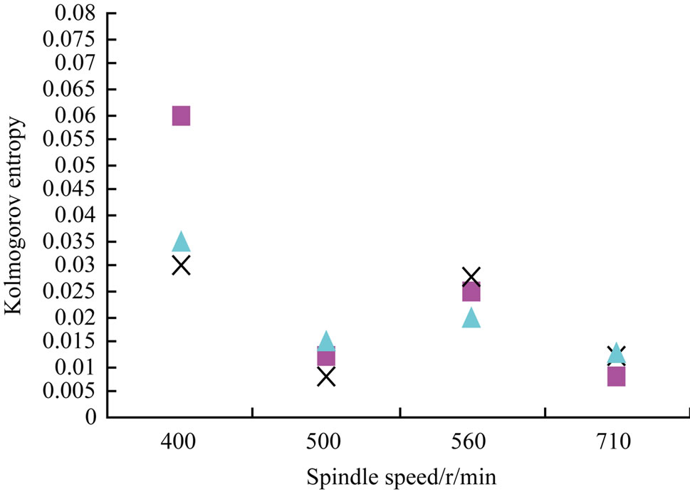 (b)
(b)
Figure 11. The plots for Lyapunov exponent and entropy versus the depth of cut; feed is 0.08 mm/r, the depth of cut is 0.6 mm. (a) Lyapunov exponent versus spindle speed; (b) Kolmogorov entropy versus spindle speed.
the stability lobes that different integration of process parameters can result in a different cutting state. The same situation from Figures 9-11 can be found. They show us the relationship between the uncertainty of cutting vibration and different integration of cutting process parameters.
Figures 9-11 display the change of the Lyapunov exponent and Kolmogorov entropy with the change of cutting conditions. We can observe the same trend in each curve. However, those figures have not display a regular effective characteristic. In an actual cutting process, even all cutting conditions are the same except the location of workpiece, the systematic motion state and the degree of chaotic characteristic in each state will be different. By analyzing the amplitude of the collected data, we can find that the amplitudes are higher when chaotic characteristic is stronger. As shown in Figure 9, the amplitude with feed 0.09 mm is 1600 mv, which is higher than the adjacent data amplitude (1400 mv). We can also see in Figure 10 that the amplitude with depth 0.3 mm is 1500 mv, which is higher than the amplitude (1200 mv) with depth 0.7 mm. The same phenomenon is found in Figure 11. Then, can we speculate the relationship between the systematic motion amplitudes and the degree of chaotic characteristics?
We can receive a variety of different data with the change of feed, cutting depth, spindle speed and the location of cutting workpiece. Calculate the Lyapunov exponent and Kolmogorov entropy of those sets of data respectively and arrange them in accordance with the order of the chatter stability amplitude from small to large, and the amplitude changes curves are drawn as shown in Figure 12, we can find with the logarithmic trend line of two sets of data that the Lyapunov exponent and Kolmogorov entropy ascend with the increase of amplitudes, which means the chaotic characteristics of systematic motion are enhanced with the increase of amplitudes.
6. Results and Discussion
We try to find some dynamic characteristics associated with the chatter formation process in this research. Specifically, we are interested in chaos or dynamical uncertainty. We divided the acquired vibration acceleration signal into three parts, chatter free, transition, and chatter processes. The signal of the transition process is in a unsteady state and cannot be digitally computed, so we studied the kinetic characteristics of the chatter-free and the chatter processes only. Both quantitative and qualitative research show that the Lyapunov exponent and the Kolmogorov entropy are on the rise from chatter-free to chatter. It shows that the irregular vibration of the cutting system is strengthening. In other words, chaos information of the cutting system is strengthening.
In this paper, we carried out experiments with different process parameters. Through the experiments we found the relationship between Lyapunov exponent and Kolmogorov entropy and process parameters behave like the stability threshold figure. If we say that the stability threshold map can assist the engineering technicians choose stable cutting parameters, then the relation curve among Lyapunov exponent and Kolmogorov entropy and the process parameters obtained in this paper can assist us to choose the best process parameters. According to this figure we can choose the best cutting parameters which can minimize the uncertainty of the cutting vibration, and reduce the vibration irregularity of the machined workpiece surface, and then obtain a higher precision.
Physical Interpretation
The phase space is  which is structured by experimental data of computing Lyapunov exponent and Kolmogorov entropy. T is Workpiece period of rotation. If the striation on the workpiece surface produced by vibration in the previous cutting can generate continuously modulating action on the striation of the workpiece surface in the subsequent cutting, then the reconstruction phase trajectory and the Lyapunov exponent and Kolmogorov entropy will be changed. Figures 5, 7 and 8 reflect the kinetic characteristics from chatter-free to chatter process. It is well known that process parameters like spindle speed, back cutting depth, and feeding speed are closely related to the stability of the cutting system. Most literatures use the threshold figure to illustrate the correlation. The drawing of the threshold figure is based on state information. The threshold figure cannot reflect the status characteristics but only the process characteristic. However, the Lyapunov exponent andKolmogorov entropy in reconstructing the phase space not only reflect the dynamic system state information but also reflect the evolutionary process information. Figures 9-11 show that Lyapunov exponent and Kolmogorov entropy have indeed changed with the changes of process parameters in cutting systems, but there is no clear patterns, such as increased or decreased trend with the increase of the process parameters. However, we can see that Lyapunov exponent and Kolmogorov entropy increase with the increase of the amplitude. In other words, chaos motion characteristics of the system increase with the increase of the amplitude from the trend line in Figure 12. We believe that the reason is: the greater the motion amplitude in the processing, the stronger influence of nonlinear factors there is, and therefore the stronger chaos characteristics. In this
 (a)
(a) (b)
(b)
Figure 12. The plots for Lyapunov exponent and entropy versus the depth of cut; feed is 0.08 mm/r, the depth of cut is 0.6 mm. (a) lyapunov exponent versus spindle speed; (b) the Kolmogorov entropy versus spindle speed.
paper, in the phase space which was built based on experimental data, we make use of Lyapunov exponent and Kolmogorov entropy tracking the changes of the dynamics characteristics of the cutting system during the transformation process from the chatter-free to the chatter.
REFERENCES
- S. A. Tobias, “Machine Tool Vibration,” Blackie, London, 1965.
- I. Koenigsberger and J. Tlusty, “Structures of Machine Tools,” Pergamon Press, Oxford, 1971.
- H. E. Merritt, “Theory of Self-Excited Machine Tools Chatter,” Journal of Engineering for Industry-Transactions of the ASME, Vol. 87, 1965, pp. 447-454.
- N. H. Hanna and S. A. Tobias, “A Theory of Nonlinear Regenerative Chatter,” ASME Journal of Engineering for Industry-Transactions, Vol. 96, 1974, pp. 247-255. doi:10.1115/1.3438305
- H. M. Shi, S. A. Tobias, “Theory of Finite Amplitude Machine Tool Instability,” International Journal of Machine Tool Design and Research, Vol. 1, No. 24, 1984, pp. 45-60. doi:10.1016/0020-7357(84)90045-3
- J. Tlusty and F. Ismal, “Basic Nonlinearity in Machining Chatter,” Annals of the CIRP, Vol. 30, No. 1, 1981, p. 299. doi:10.1016/S0007-8506(07)60946-9
- I. Grabec, “Chaos Generated by the Cutting Process,” Physics Letters, Vol. 117, No. 8, 1986, pp. 384-386. doi:10.1016/0375-9601(86)90003-4
- I. Grabec, “Chaotic Dynamics of the Cutting Process,” International Journal of Machine Tools Manufacturing, Vol. 28, 1988, pp. 19-32. doi:10.1016/0890-6955(88)90004-1
- I. Grabec, “Explanation of Random Vibrations in Cutting on Grounds of Deterministic Chaos,” Robotics and Computer& Integrated Manufacturing, Vol. 4, 1988, pp. 129-134. doi:10.1016/0736-5845(88)90067-1
- R. F. Gans, “When Is Cutting Chaotic?” Journal of Sound and Vibration, Vol. 1, No. 188, 1995, pp. 75-83. doi:10.1006/jsvi.1995.0579
- J. Gradisek, E. Govekar and I. Grabec, “A Chaotic Cutting Process and Determining Optimal Cutting Parameter Values Using Neural Networks,” International Journal of Machine Tools and Manufacture, Vol. 10, No. 36, 1996, pp. 1161-1172. doi:10.1016/0890-6955(96)00007-7
- J. Gradisek, E. Govekar and I. Grabec, “Time Series Analysis in Metal Cutting: Chatter Versus Chatter-Free Cutting,” Mechanical Systems and Signal Processing, Vol. 6, No. 12, 1998, pp. 839-854. doi:10.1006/mssp.1998.0174
- S. T. S. Bukkapatnam, A. Lakhtakia and S. R. T. Kumara, “Analysys of Sensor Signals Shows Turning on a Lathe Exhibits Low-Dimensional Chaos,” Physical Review E, Vol. 3, No. 52, 1995, pp. 2375-2378. doi:10.1103/PhysRevE.52.2375
- T. Insperger, D. A. W. Barton and G. Stepan, “Criticality of Hopf Bifurcation in State-Dependent Delay Model of Turning Process,” International Journal of Nonlinear Mechanics, Vol. 43, No. 2, 2008, pp. 140-149. doi:10.1016/j.ijnonlinmec.2007.11.002
- A. Wolf, J. B. Swift, H. L. Swinney and J. A. Vastano, “Determining Lyapunov Exponents from a Time Serie,” Physica D, Vol. 16, 1985, pp. 285-317. doi:10.1016/0167-2789(85)90011-9
- P. Grassberger and T. Procaccia, “Estimation of the Kolmogorov Entropy from a Chaotic Signal,” Physical Review A, Vol. 28, No. 4, 1983, pp. 2591-2593. doi:10.1103/PhysRevA.28.2591
- M. T. Rosensteiin, J. J. Collins, et al., “A Practical Method for Calculating Largest Lyapunov Exponents from Small Data Sets,” Journal of Physics D, Vol. 65, No. 1-2, 1993, pp. 117-134.
- H. Kantz and T. Schreiber, “Nonlinear Time Series Analysis,” Cambridge University Press, Cambridge, 1997.
- C. S. Hsu, “Probabilistic Theory of Nonlinear Dynamical Systems Based on the Cell State Space Concept,” Journal of Applied Mechanics, Transactions ASME, Vol. 4, No. 49, 1982, pp. 895-902. doi:10.1115/1.3162633
- F. C. Mooon, “Chaotic Vibrations—An Introduction for Applied Scientist and Engineers,” John Wiley& Sons, Hoboken, 1987.
- H. Kantz, “A Robust Method to Estimate the Maximal Lyapunov Exponent of a Time Series,” Physics Letters A, Vol. 185, No. 1, 1994, pp. 77-87. doi:10.1016/0375-9601(94)90991-1
- L. M. Hively and V. A. Protopopescu, “Machine Failure Forewarning via Phase-Space Dissimilarity Measures,” Chaos, Vol. 2, No. 14, 2004, pp. 408-420.