Journal of Mathematical Finance
Vol.06 No.01(2016), Article ID:63967,11 pages
10.4236/jmf.2016.61017
Extended Correlations in Finance
Mark Burgin1, Gunter Meissner2,3,4
1UCLA Department of Mathematics, Los Angeles, CA, USA
2Derivatives Software, www.dersoft.com
3Cassandra Capital Management, www.cassandracm.com
4MathFinance at NYU-Courant, New York, USA

Copyright © 2016 by authors and Scientific Research Publishing Inc.
This work is licensed under the Creative Commons Attribution International License (CC BY).
http://creativecommons.org/licenses/by/4.0/


Received 9 November 2015; accepted 24 February 2016; published 29 February 2016
ABSTRACT
Extended correlations, i.e. correlations that can take values less than −1 and/or larger than 1, occur naturally in mathematical models of financial processes. Extended correlations also occur in financial practice, especially in dispersion trading, implying arbitrage opportunities. Based on theoretical and practical emergence of extended correlations, we derive a mathematical framework for extended correlations explaining interpretations and applications. We develop a broader mathematical approach, which can model conventional as well as extended correlations.
Keywords:
Extended Correlation, Pearson Correlation, Financial Process, n-Aspect Correlation Coefficient, n-Factor Correlation Coefficient, Complete Correlation Coefficient, Total Correlation Coefficient

1. Introduction
New discoveries are often met with skepticism and resistance. When negative numbers came to Europe in books of Eastern mathematicians, critics dismissed their sensibility. Many well-known European mathematicians, e.g., Jean le Rond d’Alembert (1717-1783) or Augustus De Morgan (1806-1871), rejected the sensibility of negative numbers until the 18th century and referred to them as “absurd” or “meaningless” (Kline, 1980 [1] ; Mattessich, 1998 [2] ). Even in the 19th century, it was a common practice to criticize any negative results derived from equations, on the assumption that they were meaningless (Martinez, 2006 [3] ). For instance, Lazare Carnot (1753- 1823) argued that “the attempt to take it [a number] away from a number less than itself is ridiculous”, affirming that the idea of something being less than nothing is absurd (Mattessich, 1998 [2] ). Some other outstanding mathematicians, such as William Hamilton (1805-1865) and August De Morgan (1806-1871), had similar opinions.
Likewise, irrational numbers and later imaginary numbers were firstly rejected. Today these concepts are accepted and applied in numerous scientific and practical fields, such as physics, chemistry, biology and finance.
Similarly, probabilities less than 0 and greater than 1 were long considered non-sensible. However, these extended probabilities and especially their important case-negative probabilities with values between 1 and −1, have been applied in physics for quite a while (cf. Wigner, 1932 [4] ; Dirac, 1942 [5] ; 1943 [6] ; Bartlett, 1945 [7] ; Feynman, 1987 [8] ; Mückenheim, 1986 [9] ; Krennikov, 1992 [10] and 2009 [11] ). The probabilities which are negative and bigger than 1 are also applied in finance (Haug, 2004 [12] ; Székely, 2005 [13] ; Burgin and Meissner, 2010 [14] and 2012 [15] ; and 2012 [16] ).
Mathematical patterns of negative probabilities were studied in Bartlett 1945 [7] and in Allen 1976 [17] . A mathematical theory of negative probabilities in p-adic fields was developed in (Krennikov, 2009) [11] . A mathematical theory of extended probabilities, which included negative probabilities, was created by Burgin and Meissner in 2010 [14] and 2012 [15] for the standard situations in physics, economics and finance, where real numbers and not p-adic numbers are used. Mathematically grounded interpretations of negative probabilities were constructed in Burgin, 2012 [18] ; Abramsky and Brandenburger, 2014 [19] .
In this paper, we study correlation coefficients used in mathematical models of financial markets. By their conventional construction, correlation coefficients cannot be larger than 1 and smaller than −1. However, by exploring the theory and practice of financial markets, we have discovered emergence of correlation coefficients beyond these limits. We call them extended correlations and develop a mathematical theory for them.
The significance of our research lies on the fact that conventional mathematical theories cannot fully model all existing correlation values and processes in finance. That is why we introduce and study the concept of extended correlations, which is more general than conventional correlations including them as a special case. Hence all correlations in finance (and other sciences), i.e. conventional, and correlations that are smaller than −1 or larger than 1 can be evaluated using the concept of extended correlations.
The rest of the paper is organized as follows. In Section 2, we show that extended correlations can naturally occur in mathematical models of financial processes. In Section 3, we find extended correlations in the practice of financial markets, which imply arbitrage opportunities. In Section 4, we build mathematical foundations for extended correlations. Section 5 addresses the limitations of our concept. Section 6 concludes.
2. Extended Correlations in Financial Modeling
Financial variables such as stocks, bonds, interest rates, commodities, and volatilities are stochastic, i.e. they can be only predicted with a certain probability. Therefore, it is a good idea to model financial variables with stochastic processes as it is done in mathematical finance.
Recent events, such as the global financial crisis 2007-2009, have highlighted an important critical financial variable: correlation. In the crisis, correlations between many financial variables such as stocks, bonds, loans, and especially, sub-prime mortgage loans often securitized in a CDO, increased sharply and led to large unexpected losses. Hence, “Correlation Risk”, the risk of unfavorable change in correlation, has recently been addressed in financial modeling as well as in risk management and regulation1.
It has been suggested (see Emmerich, 2006 [20] , Ma, 2009 [21] and 2009 [22] ) to model correlations with a bounded Jacobi process of the form
 (1)
(1)
where:
ρ is the Pearson correlation coefficient2,
a is the mean reversion parameter (speed, gravity) i.e. degree with which the correlation at time t,
ρt is pulled back to its long term mean mρ, 0 ≤ a ≤ 1,
σρ is the volatility of ρ; σρ > 0,
mρ is the long term mean of the correlation ρ,
h is the upper boundary level, f: lower boundary level, i.e. h ≥ ρ ≥ f,
εt is the random drawing from a standard normal distribution at time t, ε = n~(0,1).
Applying traditional Pearson correlation values, i.e. −1 ≤ ρ ≤ +1, the upper bound h becomes +1 and the lower bound f becomes −1 and Equation (1) reduces to
 (2)
(2)
For high values of the correlation volatility σρ and low values of the mean reversion parameter “a”, Equations (1) and (2) can result in correlation values ρ of < −1 and > +1, and the equations cannot be evaluated (since the
terms  and
and  cannot be evaluated). Hence we have to introduce boundary condi-
tions, which are
 and
and  (3)
(3)
for Equation (1) and
 and
and  (4)
(4)
for Equation (2).
However, there are problematic issues with Equations (1) and (2) and its boundary conditions (3) and (4). When modeling financial correlations in practice, we have to discretize Equations (1) and (2). Equations (1) and (2) then become
 (5)
(5)
 (6)
(6)
respectively.
For Equations (5) and (6) the boundary conditions (3) and (4) are invalid, i.e. even if the boundary conditions are met, it can happen that Equations (5) and (6) cannot be evaluated. This is especially the case for high correlation volatility σρ and low values of the mean reversion parameter “a”. There are several solutions to this problem:
1) We can introduce limits which the correlation values can take. The limits would be h and f for Equation (5) and −1 and +1 for Equation (6). We could compute Equation (5) as
 (7)
(7)
Equation (7) reads: If the simulated correlation coefficient at t, ρt, is smaller than the lower boundary f, take the value f; if the simulated correlation coefficient at t, ρt, is greater than the upper boundary h, take the value h,
otherwise apply Equation (5) . For Equation (6), the
lower boundary f = −1, and the higher boundary h = +1. However, the approach (7) arbitrary and model-incon- sistent.
2) We can allow extended correlations increasing the upper boundary h above +1 and decreasing the lower boundary f below −1 in Equation (5). However, increasing h and decreasing f would effectively increase the volatility of the correlation ρ since the last terms of Equations (5) and (6) are amplified.
3) A viable solution to this problem is to allow utilization of extended correlations and to describe correlation by means of a standard mean-reverting Vasicek model of the form
 (8)
(8)
or by its discrete version
 (9)
(9)
Equations (8) and (9) can be evaluated in every simulation with the standard parameter values 0 ≤ a ≤ 1 and σρ > 0.
In summary, the Jacobi process, which has been suggested to model correlation, can lead to errors when simulating discrete correlations in reality. Increasing the boundaries in a Jacobi process solves the problem, however at the cost of increased correlation volatility.a viable solution is to apply a standard Vasicek model and allow extended correlations. This will guarantee that every real-world discrete correlation simulation is executed without receiving error values.
Extended Correlations as an Input for Financial Models
In finance, the Pearson correlation coefficient or a Pearson correlation matrix serves as an input for many financial models. For example, Copulas typically apply the Pearson correlation coefficient or a Pearson correlation matrix. Due to its convenient properties, the thin-tailed Gaussian copula is often used in finance. For the bivariate Gaussian copula, the density function is
 (10)
(10)
where  and N−1 is the inverse of the standard normal distribution, and ρ is the Pearson correlation coefficient. Figure 1 and Figure 2 show the density of the bivariate copula with uniform marginals.
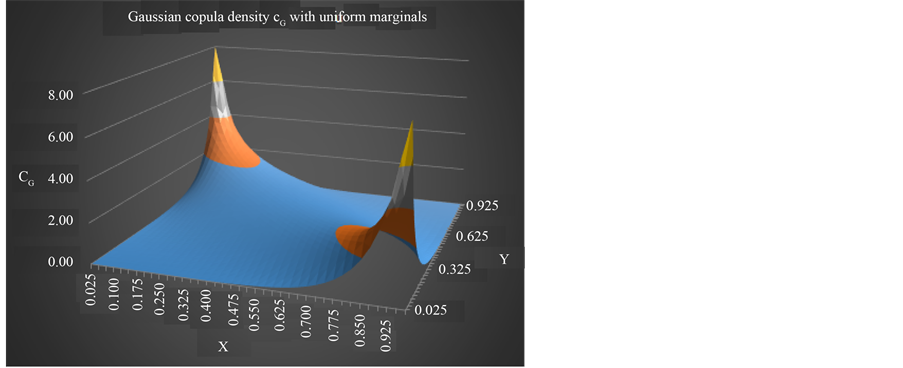
Figure 1. Gaussian copula density with ρ = −0.8.
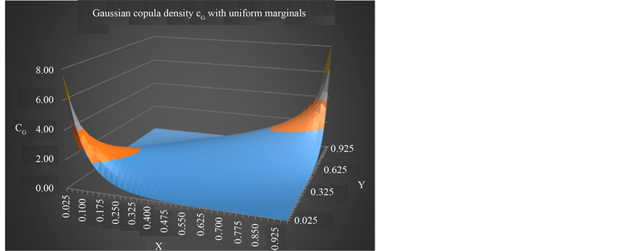
Figure 2. Gaussian copula density with ρ = +0.8.
From Figure 1 and Figure 2 we can observe the critical impact of the correlation parameter ρ on the density function.
To derive the dependency for more than two variables, often a factorization is applied. This OFGC (one-fac- tor Gaussian copula) model is
 (11)
(11)
where:
M is the systematic factor, which impacts all variables xi. As ԑ, M is a random drawing from a standard normal distribution, M = n~(0,1).
Zi is the idiosyncratic factor of entity i. Just like M, Zi is a random drawing from a standard normal distribution, Zi = n~(0,1).
xi: The variables xi for  are correlated with each other by “conditioning on M”. From Equation (11) we observe that for ρ = 1, all xi are equal to M in a certain simulation, i.e. all xi are identical. For ρ = 0, all xi are equal to their idiosyncratic factor Zi, i.e. they are independent.
The seminal Heston model applies a similar model as Equation (11). It correlates two Brownian motions dz1 and dz2 with the Pearson correlation coefficient ρ, where dz = εtdt and εt is defined as in Equation (1). The core equation is
 (12)
(12)
Numerous extensions of the Heston (1993) model exist, see for example Hagan et al. (2002) [25] and Buraschi et al. (2006) [26] .
By construction, Equations (10) to (12) limit the correlation parameter ρ to −1 ≤ ρ ≤ 1. Hence in order to apply extended correlations, we have to alter the equations. Changing the term  in Equations (11) and (12) to
  or 1 − ρ would add model flexibility. For ρ > 1, the dependent variable xi or dz1(t) have a higher than 100% positive dependence on M or dz2(t) respectively, and a negative dependency on Zi or dz3 respectively. Vice versa, for ρ < −1, the dependent variable xi or dz1(t) have a higher than 100% negative dependence on M or dz2(t) respectively, and a positive dependency on Zi or dz3 respectively. The higher flexibility comes at the cost of loss of standard normality for xi and dz1. While the mean, skewness and kurtosis of dz1 and xi would still be zero, the variance is unequal to 1 for all ρ\{0,1}. Equation (10) is not a good candidate for extended correlations since they can change the sign of the equation.
3. Extended Correlations in Financial Practice
Extended correlations occur in finance if arbitrage opportunities exist. We will show this with the example of dispersion trading.
Dispersion trading emerged in the late 1990s from index arbitrage. In a long index arbitrage trade, the trader buys certain components (e.g. stocks) of an index (e.g. the S&P 500) and shorts the whole index. The index
components are expected to outperform the index, so that  where wi are the component weights,
ri is the return of the index components and ri is the return of the Index.
Dispersion trading applies the same idea, just with respect to component volatility and index volatility. The strategy can be well implemented with options. For details on dispersion trading see Willmott (2009) [27] or Meissner (2015) [28] .
Let’s briefly derive the core equation of dispersion trading. We start with the variance equation for two assets i and j, . Generalizing for n assets, which comprise the index I, and using financial notation, i.e. Var ≡ σ2, we derive
 (13)
(13)
where  is the implied variance of the Index, i.e. the variance implied by option prices on the index, and
  is the implied variance of an option on the component i, and wi and wj are weighting factors. Solving equation (13) for the average implied pairwise correlation coefficient between assets i and j, ρij, we derive
 (14)
(14)
Equation (14) shows the general concept of dispersion trading. The correlation between the components i and j, ρij, is not derived by data points in a two-dimensional coordinate system as in the Pearson model, but by the relationship between the index implied volatility σi and component implied volatility σi.
The CBOE disseminates the implied correlation index of the S&P 500 derived by Equation (14) since 2007, ticker symbol ICJ, JCJ, and KCJ, see http://www.cboe.com/micro/impliedcorrelation. So far the CBOE has reported 3 extended correlations. Not surprisingly, they occurred at the height of the global financial crisis: On November 6, 2008, implied correlation was 100.8%, on November 13, 2008, 105.93% and on November 20, 2008, 103.04% for the KCJ, the January 2009 option maturity. This confirms that extended correlations exist in financial practice.
The extended correlations imply arbitrage opportunities: If ρij > 1, from Equation (14), we observe that implied index volatility  is too high relative to the component volatility
 . I.e. index volatility can be sold and component volatility bought realizing a risk-free profit (assuming no transaction cost, and mid-market execution). The type of arbitrage, ρij > 1, not ρij < −1, is plausible. For instance, in the severe crisis of 2008, traders assumed that many stocks would decline jointly. Hence, they bought puts on the whole index I, driving up index volatility
  to levels, which generated the correlation coefficients ρij > 1, i.e., they became not conventional but extended correlations.
In the following section, we derive a mathematical model for extended correlations constructing two basic types of extended correlation coefficients: complete correlation coefficients and total correlation coefficients.
4. A Mathematical Model for Extended Correlations
Let us first review constructions and properties of Pearson’s correlation coefficient, also called population correlation coefficient, if a whole population is modeled. For two variables X and Y, it is defined by
 (15)
(15)
where cov(X, Y) is the covariance of X and Y, while sX and sY are the standard deviations of X and Y, respectively.
If we model random variables, it is possible to express the correlation coefficient in terms of expectations
 (16)
(16)
In the case when random variables X and Y are represented by samples, the sample Pearson correlation coefficient, or sample correlation coefficient, rX,Y is defined by
 (17)
(17)
where  is a sample for X with the sample mean mx and
  is a sample for Y with the sample mean my.
The properties of the Pearson correlation coefficients are well-known:
1) The population correlation coefficient has the following boundaries
 .
.
2) The sample correlation coefficient has the same boundaries
 .
.
3) The population correlation coefficients symmetric, i.e., rX,Y = rY,X.
4) The sample correlation coefficients symmetric, i.e., rX,Y = rY,X.
5) The population correlation coefficients invariant with respect to linear transformations of the two variables, namely, changing X to a + bX and Y to c + dY, where a, b, c, and d are constants with b, d > 0, does not change the population correlation coefficient rX,Y.
6) The sample correlation coefficients invariant with respect to linear transformations of the measurement scales, i.e., of the x-y-coordinates, namely, changing the coordinate x to a + bx and the coordinate y to c + dy, where a, b, c, and d are constants with b, d > 0, does not change the sample correlation coefficient rX,Y.
7) The equality rX,Y = 1 implies that a linear equation perfectly describes the relationship between X and Y, with all data points lying on a line for which Y increases as X increases.
8) The equality rX,Y = −1 implies that a linear equation perfectly describes the relationship between X and Y, with all data points lie on a line for which Y decreases as X increases.
9) The equality rX,Y = 0 implies that there is no linear dependency between the variables X and Y.
However, as demonstrated above, to better model financial reality, it is necessary to use extended correlation coefficients. At first, we consider population correlation coefficients.
To understand how extended correlation coefficients emerge in a mathematical context, we delineate a set A of aspects of the random variables X and Y assuming that it is possible to numerically represent each aspect A from A, i.e., there are variables XA and YA that represent the aspect A in the variables X and Y.
This allows us to define the aspect population correlation coefficient for variables X and Y as
 (18)
(18)
To find an integral correlation characteristic, it is possible to use the complete population correlation coefficient for variables X and Y, which is computed by the following formula:
 (19)
(19)
When the set A consists of n aspects, the value  is called the n-aspect population correlation coefficient.
It is also possible to use the aspect sample correlation coefficient for variables X and Y
 (20)
(20)
Then the complete sample correlation coefficient for variables X and Y is based on the aspect sample correlation coefficients and is computed by the following formula:
 (21)
(21)
When the set A consists of n aspects, the value  is called the n-aspect sample correlation coefficient.
Example 1. Let us consider a situation when a company wants to find the correlation between its profit and expenses. The company has three factories and wants to take into account all of them. To find the necessary correlation, a statistician represents the profit by the random variable X and the expenses by the random variable Y. Each factory represents a factor of these variables. Then it’s possible to use the complete correlation coefficient, which better represents relations between profit and expenses than the conventional correlation coefficient.
In this case, the profit of the first factory is represented by the random variable X1 and the expenses related to the first factory - by the random variable Y1. The profit of the second factory is represented by the random variable X2 and the expenses related to the second factory-by the random variable Y2. The profit of the first factory is represented by the random variable X3 and the expenses related to the first factory-by the random variable Y3. Then the complete (or 3-aspect) sample correlation coefficient for variables X and Y is equal to

For instance,  ,
,  , and
, and . In this case, the complete sample correlation coefficient
 .
.
If ,
,  , and
, and . In this case, the complete sample correlation coefficient
 .
.
If ,
,  , and
, and . In this case, the complete sample correlation coefficient
 .
.
Example 2. Let us consider a situation when a biologist wants to find correlation between traits of fathers and sons. Then it possible to use the complete correlation coefficient taking such features as the height, weight, color of eyes, IQ and education in the role of aspects of the compared trait.
In this case, the height of the father is represented by the random variable X1 and the height of the son―by the random variable Y1. The weight of the father is represented by the random variable X2 and the weight of the son―by the random variable Y2. The IQ of the father is represented by the random variable X3 and the IQ of the son by the random variable Y3. In addition, it is possible to assign numerical values to the color of eyes and education, for example, assigning 0 to the case when a person does not have any education and 10 when a person has PhD. This makes possible representation of father’s color of eyes by the random variable X4 and son’s color of eyes by the random variable Y4. In a similar way, we represent father’s education by the random variable X5 and son’s education by the random variable Y5.
Then the complete sample correlation coefficient for variables X and Y is equal to

For instance,  ,
,  ,
,  ,
,  , and
, and . In this case, the complete (or 5-aspect) sample correlation coefficient
 .
.
Some properties of complete correlation coefficients are the same as properties of conventional correlation coefficients, while other properties are different. Based on the properties 1 - 8 of conventional correlation coefficients considered above, we obtain the following results.
1) The complete (n-aspect) population correlation coefficient  has the following boundaries
 .
.
2) The complete (n-aspect) correlation coefficient  has the same boundaries
 .
.
3) The complete (n-aspect) population correlation coefficient is symmetric, i.e., .
.
4) The complete (n-aspect) sample correlation coefficient is symmetric, i.e.,  .
.
5) The complete (n-aspect) population correlation coefficient is invariant with respect to linear transformations of the two variables and their aspects, namely, changing X to a + bX and Y to c + dY, where a, b, c, and d are constants with b, d > 0, does not change the complete population correlation coefficient .
.
6) The complete (n-aspect) sample correlation coefficient is invariant with respect to linear transformations of the measurement scales, i.e., of the x-y-coordinates, namely, changing the coordinate x to a + bx and the coordinate y to c + dy, where a, b, c, are constants with b, d > 0, does not change the complete sample correlation coefficient  .
.
7) The equality  implies that a linear equation perfectly describes the relationship between all corresponding aspects of X and Y, with all data points lying on a line for which the aspect of Y increases as the corresponding aspect of X increases.
8) The equality  implies that a linear equation perfectly describes the relationship between all corresponding aspects of X and Y, with all data points lying on a line for which the aspect of Y decreases as the corresponding aspect of X increases.
Proofs of these properties are based on the properties 1 - 8 of conventional correlation coefficients.
Another way to build extended correlation coefficients is based on factors of random variables. Let us assume that we have a set F of factors of the random variables X and Y assuming that it is possible to numerically represent each factor F from F, i.e., there are variables XF and YF that represent the factor A in the variables X and Y.
This allows us to define the factor population correlation coefficient for variables X and Y as
 (22)
(22)
To find an integral correlation characteristic, it is possible to use the total population correlation coefficient for variables X and Y, which is computed by the following formula:
 (23)
(23)
When the set F consists of n factors, the value  is called the n-factor population correlation coefficient.
It is also possible to use the factor sample correlation coefficient for variables X and Y
 (24)
(24)
Then the total sample correlation coefficient for variables X and Y is based on the factor sample correlation coefficients and is computed by the following formula:
 (25)
(25)
Example 3. Let us consider a situation when an investor wants to find correlation between prices of stocks of companies A and B. Then it possible to use the total correlation coefficient, taking into account factors that influence prices of stocks, which could be the PE (price earnings ratio), EPS (earnings per share), and the dividend yield. This allows achieving better representation of dependencies than the conventional correlation coefficient.
In this case, the PE of the company A is represented by the random variable X1 and the PE of the company B- by the random variable Y1. The EPS of the company A is represented by the random variable X2 and the EPS of the company B- by the random variable Y2. The dividend yield of the company A is represented by the random variable X3 and the dividend yield of the company B-by the random variable Y3. Then the total (or 3-aspect) sample correlation coefficient for variables X and Y is equal to

For instance,  ,
,  , and
, and . In this case, the complete sample correlation coefficient
 .
.
If ,
,  , and
, and . In this case, the complete sample correlation coefficient
 .
.
If ,
,  , and
, and . In this case, the complete sample correlation coefficient
 .
.
Some properties of total correlation coefficients are the same as properties of conventional correlation coefficients, while other properties are different. Based on the properties 1 - 8 of conventional correlation coefficients considered above, we obtain the following results.
1) The total (n-factor) population correlation coefficient has the following boundaries
 .
.
2) The total (n-factor) sample correlation coefficient has the same boundaries
 .
.
3) The total (n-factor) population correlation coefficient is symmetric, i.e., .
.
4) The total (n-factor) sample correlation coefficient is symmetric, i.e., .
.
5) The total (n-factor) population correlation coefficient is invariant with respect to linear transformations of the two variables, namely, changing X to a + bX and Y to c + dY, where a, b, c, and d are constants with b, d > 0, does not change the total population correlation coefficient .
.
6) The total (n-factor) sample correlation coefficient is invariant with respect to linear transformations of the measurement scales, i.e., of the x-y-coordinates, namely, changing the coordinate x to a + bx and the coordinate y to c + dy, where a, b, c, and d are constants with b, d > 0, does not change the total sample correlation coefficient .
.
7) The equality  implies that a linear equation perfectly describes the relationship between all corresponding factors of X and Y, with all data points lying on a line for which the factor of Y increases as the corresponding factor of X increases.
8) The equality  implies that a linear equation perfectly describes the relationship between all corresponding factors of X and Y, with all data points lying on a line for which the factor of Y decreases as the corresponding factor of X increases.
Proofs of these properties are based on the properties 1 - 8 of conventional correlation coefficients.
5. Limitations of the Model
The correlations, which are created in this paper, are extended from the Pearson correlation model. While the Pearson correlation model is by far the most applied correlation model in finance, it suffers from several limitations. The main limitations are
1) The Pearson can only evaluate linear associations between variables
2) As a consequence of 1), The Pearson coefficients can only be meaningfully interpreted if the data distribution is approximately elliptical.
3) Outliers can distort the correlation results
4) Different time frames can lead to very different results
5) The causality has to be determined exogenously
6) Spurious correlation can occur
For a detailed discussion on ten limitations of the Pearson model, see Meissner 2015 [14] . These limitations are inherited by the new model.
6. Conclusions
When modeling financial processes with discrete stochastic processes, extended correlations, i.e. correlations which can be <−1 and >1, naturally occur. Rather than discarding the whole model or applying arbitrary boundaries, extended correlations can be implemented to utilize the model.
Correlations often serve as an input for more complex mathematical models such as copulas or Heston models. Utilization of extended correlations in these models adds flexibility such as extending of the dependencies between variables beyond unity.
Extended correlations occur in financial practice as the 2008 global financial crisis demonstrated. Consequently, there is a need to create a sound mathematical model for extended correlations.
We derive one type of extended correlation coefficients by delineating a set A of aspects of random variables and creating aspect correlation coefficients and combining them into the complete, or n-aspect, correlation coefficient. Some properties of the complete correlation coefficient are different from the traditional Pearson correlation coefficient, for example, boundaries of the coefficient become −n and +n, while other properties, such as symmetry, remain unchanged.
Another way to build extended correlation coefficients is based on factors of random variables. Taking a factor F from a set F, which consists of n factors of considered processes, we build the quantity  called a factor correlation coefficient and combine factor correlation coefficients into the total, or n-factor, correlation coefficient. As with the complete correlation coefficient, the total correlation coefficient can have wider boundaries, while some of its properties are identical to the Pearson correlation coefficient.
In conclusion, conventional mathematical correlation approaches cannot fully model all existing correlation values and processes. Therefore we introduce the model of extended correlations, which is more general than the conventional correlation models. Hence all correlations in finance (and other sciences), i.e. conventional, and correlations that are smaller than −1 or larger than 1, can be represented by extended correlations.
Cite this paper
MarkBurgin,GunterMeissner,11,11, (2016) Extended Correlations in Finance. Journal of Mathematical Finance,06,178-188. doi: 10.4236/jmf.2016.61017
References
- 1. Kline, M. (1980) Mathematics: The Loss of Certainty. Oxford University Press, New York.
- 2. Mattessich, R. (1998) From Accounting to Negative Numbers: A Signal Contribution of Medieval India to Mathematics. Accounting Historians Journal, 25, 129-145
- 3. Martinez, A.A. (2005) Negative Math: How Mathematical Rules Can Be Positively Bent. Princeton University Press.
- 4. Wigner, E.P. (1932) On the Quantum Correction for Thermodynamic Equilibrium. Physics Review, 40, 749-759.
http://dx.doi.org/10.1103/physrev.40.749 - 5. Dirac, P.A.M. (1942) The Physical Interpretation of Quantum Mechanics. Proceedings of the Royal Society of London, 180, 1-39.
http://dx.doi.org/10.1098/rspa.1942.0023 - 6. Dirac, P.A.M. (1943) Quantum Electrodynamics. Communications of the Dublin Institute for Advanced Studies.
- 7. Bartlett, S. (1945) Negative Probability. Mathematical Proceedings of the Cambridge Philosophical Society, 41, 71-73.
http://dx.doi.org/10.1017/S0305004100022398 - 8. Feynman, R. (1987) Negative Probability. In: Hiley, B.J. and Peat, F., Eds., Quantum Implications: Essays in Honour of David Bohm, Routledge & Kegan Paul Ltd., London and New York, 235-248.
- 9. Mückenheim, W., Ludwig, G., Dewdney, C., Holland, P.R., Kyprianidis, A., Vigier, J.P., et al. (1986) A Review of Extended Probabilities. Physics Reports, 133, 337-401.
http://dx.doi.org/10.1016/0370-1573(86)90110-9 - 10. Khrennikov, A. (1992) p-Adic Probability and Statistics. Dokl. Acad. Nauk, 322, 1075-1079.
- 11. Khrennikov, A. (2009) Interpretations of Probability. Walter de Gruyter, Berlin/New York.
http://dx.doi.org/10.1515/9783110213195 - 12. Haug, E.G. (2004) The Collector: Why So Negative to Negative Probabilities? Wilmott Magazine, 34-38.
- 13. Székely, G.J. (2005) Half of a Coin: Negative Probabilities. Wilmott Magazine, 66-68.
- 14. Burgin, M. and Meissner, G. (2010) Negative Probabilities in Modeling Random Phenomena. Integration: Mathematical Theory and Application, 2, 305-322.
- 15. Burgin, M. and Meissner, G. (2012) Larger Than One Probabilities in Mathematical and Practical Finance. Review of Economics and Finance, No. 4, 1-13.
- 16. Burgin, M. and Meissner, G. (2012) Negative Probabilities in Financial Modeling. Wilmott Magazine, 58, 60-65.
- 17. Allen, E.H. (1976) Negative Probabilities and the Uses of Signed Probability Theory. Philosophy of Science, 43, 53-70.
http://dx.doi.org/10.1086/288669 - 18. Burgin, M. (2012) Integrating Random Properties and the Concept of Probability. Integration: Mathematical Theory and Applications, 3, 137-181.
- 19. Abramsky, S. and Brandenburger, A. (2014) An Operational Interpretation of Negative Probabilities and No-Signalling Models. Lecture Notes in Computer Science, 8464, 59-75.
http://dx.doi.org/10.1007/978-3-319-06880-0_3 - 20. Emmerich, C. (2006) Modeling Correlation as a Stochastic Process. Working Paper, Bergische Universitaet, Wuppertal.
- 21. Ma, J. (2009) Pricing Foreign Equity Options with Stochastic Correlation and Volatility. Annals of Economics and Finance, 10, 303-327.
- 22. Ma, J. (2009) A Stochastic Correlation Model with Mean Reversion for Pricing Multi-Asset Options. Asia Pacific Financial Markets, 16, 97-109.
- 23. Basel Committee of Banking Supervision (2009) Principles of Sounds Stress Testing Practices and Supervision. BCBS, Basel.
- 24. Meissner, G. (2015) The Pearson Correlation Model—Work of the Devil? Working Paper.
- 25. Hagan, P.S., Kumar, D., Lesniewski, A.S. and Woodward, D.E. (2002) Managing Smile Risk. Wilmott Magazine, 84-108.
- 26. Buraschi, A., Porchia, P. and Trojani, F. (2006) Correlation Risk and Optimal Portfolio Choice. Journal of Finance, 65, 392-342.
http://dx.doi.org/10.2139/ssrn.908664 - 27. Wilmott, P. (2009) Frequently Asked Question in Quantitative Finance. John Wiley, Hoboken.
- 28. Meissner, G. (2015) Correlation Trading—Opportunities and Limitations. Working Paper.
NOTES

1For example the Basel accord addresses several correlation measures as “general and specific wrong-way risk”, and the stress testing of correlations, see [23] Basel Committee of Banking Supervision “Principles of sounds stress testing practices and supervision” May 2009.
2The Pearson correlation model can be found in virtually every descriptive statistics or econometrics textbook. For a discussion of the limitations of the Pearson model, see [24] Meissner 2015.