Applied Mathematics
Vol.4 No.6(2013), Article ID:33439,5 pages DOI:10.4236/am.2013.46132
Simulations of Rayleigh’s Wave on Curved Surface
1Institute of Applied Mathematics, National Cheng-Kung University, Taiwan
2Department of Mechanical Engineering, Cheng Shiu University, Taiwan
Email: *shen@mail.ncku.edu.tw
Copyright © 2013 Shih-Yu Shen, Chin-Yu Wang. This is an open access article distributed under the Creative Commons Attribution License, which permits unrestricted use, distribution, and reproduction in any medium, provided the original work is properly cited.
Received March 15, 2013; revised April 11, 2013; accepted April 21, 2013
Keywords: Elastodynamics; Lamb’s Problem; Boundary Element Method; Rayleigh’s Wave
ABSTRACT
Impulsive line load in a half-space (Lamb’s problem) can be solved with a closed form solution. This solution is helpful for understanding the phenomenon of Rayleigh’s waves. In this article, we use a boundary element method to simulate the solution of an elastic solid with a curved free surface under impact loading. This problem is considered difficult for numerical methods. Lamb’s problem is calculated first to verify the method. Then the method is applied on the problems with different surface curvatures. The method simulates the phenomenon of Rayleigh’s wave propagating on a curved surface very well. The results are shown in figures.
1. Introduction
The phenomenon of surface wave is interesting and important for many engineers and scientists. Impulsive line load in a half-space can be solved by analytic methods [1]. Herewith scientists and engineers may get understanding with Rayleigh’s wave. When the free surface is not flat the phenomenon of surface wave should be similar, but some detail can be different. On the case of curved surface, analytic solutions are no longer available. Therefore numerical methods become an alternative way to understand the phenomena. These problems are considered difficult for numerical methods. To the best of our knowledge, there are no related reports on this problem.
Simulating transient wave in elastodynamics needs mass computing time and huge memories. Boundary element methods are efficient for simulating elastodynamics [2,3]. Recently personal computers (PC) become much more powerful and are equipped with more rams then ever. Practical problems can be simulated with a PC precisely.
In this article, we use a boundary element method to solve two dimensional elastodynamic problems with curved surfaces. The curved boundary is assumed to be an arc. The loading is an impulse. The numerical method is implemented with fortran programs and a PC. In Section 2, the mathematical problem is described. In the following section, we formulate the numerical method briefly. The results are shown in Section 4.
2. The Problem
Because our goal is to simulate the Rayleigh wave on a smooth surface near the loading point, the boundary of the 2D domain ![]() is modeled as a arc with curvature
is modeled as a arc with curvature
 . The loading is a single line impact at the surface.
The schematic diagram is shown in Figure 1.
Boundary value problems with zero initial conditions and absent body force for 2D elastodynamics in plane
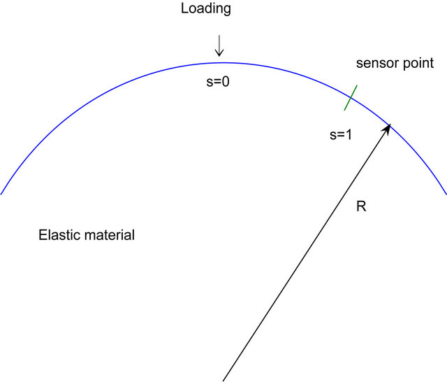
Figure 1. The schematic diagram of the geometry of the problem.
strain condition are considered. The material is homogeneous, isotropic and linear elastic.
Therefore, the displacement 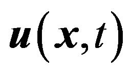 fulfills Navier’s equation; i.e.
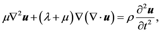 (1)
(1)
where  and
and ![]() are the Lame constants and
are the Lame constants and  is the mass density of the elastic material.
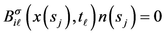
The boundary conditions are
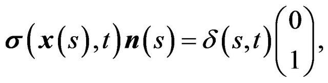 (2)
(2)
where ![]() is the stress tensor,
is the stress tensor,  is the outward normal vector on
![]() ,
, ![]() is the coordinate on the boundary,
is the coordinate on the boundary,  is the Dirac delta function, and
  presents the map from coordinate
 ![]() to 2D spatial coordinates
to 2D spatial coordinates
 . Here,
 . The time-varied displacements on the curved surface are Rayleigh’s waves.
3. The Method
We use a boundary element method to calculate the surface displacements. The boundary ![]() is approximated as a polygon.
is approximated as a polygon.
There are two families of particular solutions of Navier’s equation,  and
and .
.
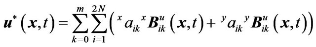
Then, the approximated displacements field are
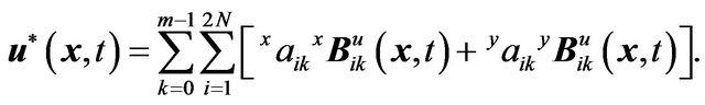 (3)
(3)
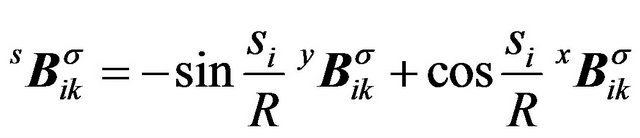
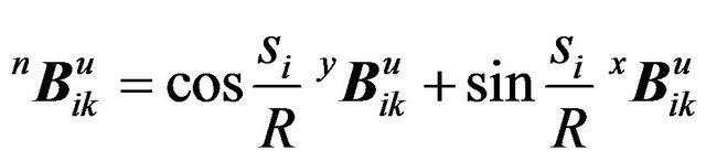
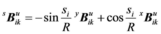
Using Hooke’s law, we have stress bases,  and
and  i.e.
i.e.
 (4)
(4)
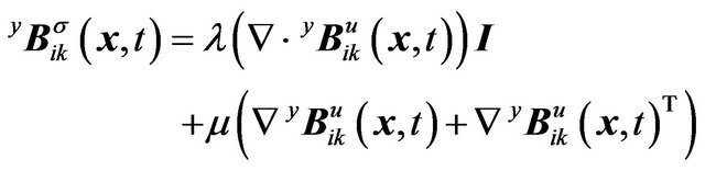 (5)
(5)
Note that  are vector fields and
  are tensor fields.
The bases ,
, ,
, and
and  have been derived in a close form [4]. The the coefficients,
  and
and , will determined with the boundary condition (2).
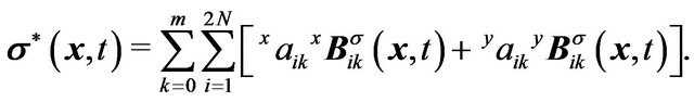
Then, the approximated stress field is
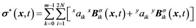 (6)
(6)
Substituting Equation (6) into boundary condition (2), we have
 (7)
(7)
When a collocation method apply on Equation (7), the coefficients  are as many as
 . It is difficult to calculate a precise elastodynamic solution on a personal computer with this formulation. Therefore we take the advantage of the symmetry of the boundary.
Let
 (8)
(8)
 (9)
(9)
and
 (10)
(10)
 (11)
(11)
 (12)
(12)
 (13)
(13)
Substituting Equations (8) and (9) into (7), we have
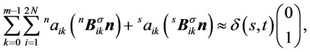 (14)
(14)
Then, we decomposite the traction into normal and tangent directions.
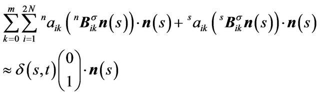 (15)
(15)
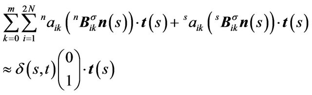 (16)
(16)
where  and
and  are normal and tangent vectors at s respectively, and
  denote the inner product of two vectors.
Let  and
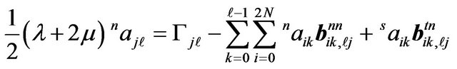
and . Then apply the semicollocation method [4] to Equations (15) and (16). Rearranging the equations for
  and
and , we have the stepping equations.
 (17)
(17)
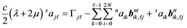 (18)
(18)
where
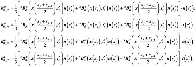 (19)
(19)
and
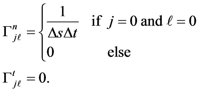 (20)
(20)
The  is approximated by
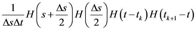 where H is the Heaviside step function.
In formulae (17) and (18), the coefficients ![]() take the form of
take the form of . The usage of computer memory is enormously deduced to 2Nm.
When ,
,  , if
, if . Thus Equations (17) and (18) are uncoupled. Thus, the timestepping scheme is explicit.
Then the time-stepping technique is applied on Equations (17) and (18) to solve  and
and  on
on  th step.
After solving the coefficients,  and
and , the numerical displacement may be calculated by
 (2.11)
and the numerical interior stress by
 (21)
(21)
4. The Results
In order to verify this method, we calculate the problem with very large  first. For
 , the problem becomes Lamb’s problem in which the exact surface displacements are available. The elastic half space
is loaded at  by a unit line impulse at
 .
.
The solutions for problems of a line impulse load on an elastic half plane were derived by Lamb. A modern treatment with integral transform technique was given by De Hoop, but the results were in complex function form. Nevertheless explicit form for surface displacements are available. The analytic solution for surface displacement can be found in page. 614-626 of [1].
The schematic diagram of the geometry of the problem is shown in Figure 1.
In this example Poisson’s ratio . Therefore the shear and Rayleigh’s wave speeds are
  and
and  respectively, where
  is the dilatation wave speed.
Figure 2 shows the displacements with vertical loading when . The dashed line shows exact displacement when
 . There is a Dirac delta function at the Rayleigh wave front in the exact solution. The vertical line indicate the arriving time of Rayleigh’s wave. For this figure,
 . Even though this problem is considered difficult for numerical methods, our results are precise. This example shows the method is applicable for impact problems.
When , the results are shown in Figure 3. In this case tangential displacement is almost the same with Lamb’s problem, but the normal displacement is changed much. The normal displacement has a strong and short peak at the shear wave front and the head wave is enlarged. The head wave is the wave beyond the shear wave front [5]. The dashed line is the displacement for
 . Figure 4 shows the displacements for
 . The phenomenon is similar to the case of
 .
.
5. Conclusion
We use the boundary element method and write a fortran program running on a personal computer. In order to simulate the phenomenon of Rayleigh’s wave propagating on a curved surface, the free surface is assumed to be a constant, . The method is verified by the problem of
 . Two examples, R = 5 and R = 3, calculated to demonstrate the phenomenon. On the shear wave front,
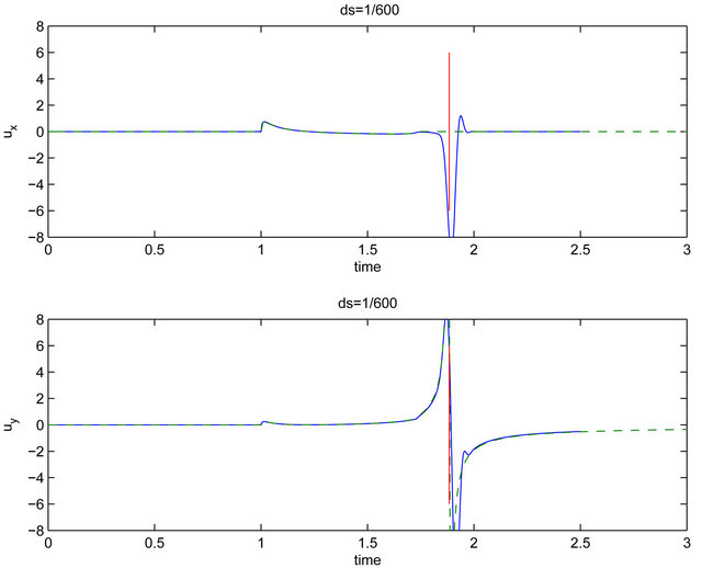
Figure 2. The displacements with vertical loading when R = 1000. The dashed line shows exact displacement when R = ∞. The vertical red lines indicate the arrival time of Rayleigh’s wave. There is a Dirac delta function at the Rayleigh wave front in the exact solution. In this figure,  is used.
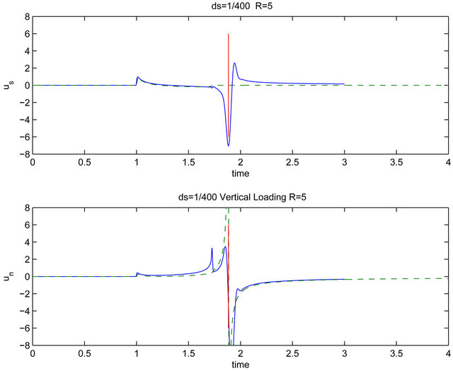
Figure 3. The displacements when R = 5. The dashed line shows exact displacement when R = ∞. The vertical red lines indicate the arrival time of Rayleigh’s wave. In this figure,  is used.
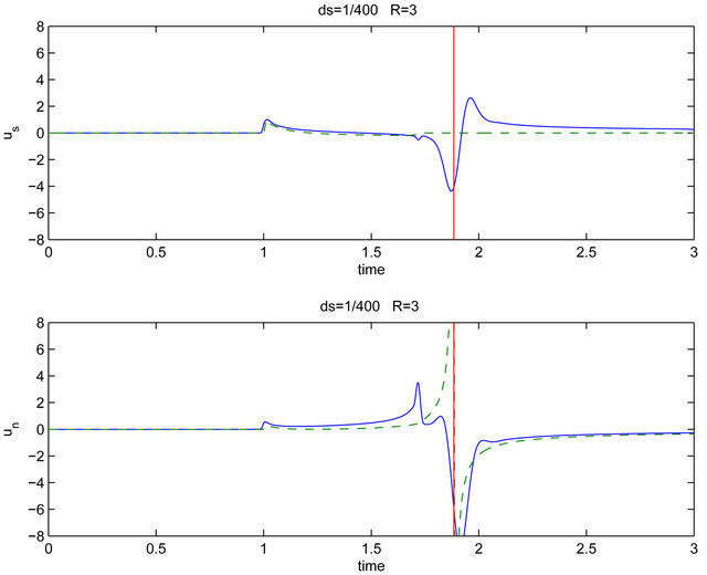
Figure 4. The displacements when R = 3. The red line shows exact displacement when R = ∞. The vertical dashed lines indicate the arrival time of Rayleigh’s wave. In this figure,  is used.
the wave is very different from that of Lamb’s problem.
REFERENCES
- A. C. Eringen and E. S. Suhubi. “Elastodynamics, Volume II,” Academic Press, New York, 1975.
- D. E. Beskos, “Boundary Element Method in Dynamic Analysis,” Applied Mechanics Review, Vol. 40, No. 1, 1987, pp. 1-23. doi:10.1115/1.3149529
- D. E. Beskos, “Boundary Element Method in Dynamic Analysis: Part II (1986-1996),” Applied Mechanics Review, Vol. 50, No. 3, 1997, pp. 149-197. doi:10.1115/1.3101695
- S. Y. Shen, “An Indirect Elastodynamics Boundary Element Method with Analytic Bases,” International Journal for Numerical Methods in Engineering, Vol. 57, No. 6, 2003, pp. 767-794. doi:10.1002/nme.702
- J. D. Achenbach, “Wave Propagation in Elastic Solid,” Noth-Holland, Amsterdam, 1976.
NOTES
*Corresponding author.