Journal of Environmental Protection
Vol.4 No.8(2013), Article ID:35695,8 pages DOI:10.4236/jep.2013.48099
Rating Curve Estimation of Surface Water Quality Data Using LOADEST
![]()
Department of Civil, Architectural and Environmental Engineering, North Carolina A&T State University, Greensboro, USA.
Email: *mkjha@ncat.edu
Copyright © 2013 Bhasker Jha, Manoj Kumar Jha. This is an open access article distributed under the Creative Commons Attribution License, which permits unrestricted use, distribution, and reproduction in any medium, provided the original work is properly cited.
Received December 26th, 2012; revised February 8th, 2013; accepted April 13th, 2013
Keywords: LOADEST; Rating Curve; Nutrient Load; Water Quality
ABSTRACT
Measurement of the nutrient concentrations in the stream is usually done on weekly, biweekly or monthly basis due to limited resources. There is need to estimate concentration and loads during the period when no data is available. The objectives of this study were to test the performance of a suite of regression models in predicting continuous water quality loading data and to determine systematic biases in the prediction. This study used the LOADEST model which includes several predefined regression models that specify the model form and complexity. Water quality data primarily nitrogen and phosphorus from five monitoring stations in the Neuse River Basin in North Carolina, USA were used in the development and analyses of rating curves. We found that LOADEST performed generally well in predicting loads and observation trends with general tendency/bias towards overestimation. Estimated Total Nitrogen (TN) varied from observation (“true” load) by −1% to 9%, but for the Total Phosphorus (TP) it ranged from −2% to 27%. Statistical evaluation using R2, Nash-Sutcliff Efficiency (NSE) and Partial Load Factor (PLF) showed a strong correlation in prediction.
1. Introduction
Accurate estimation of nutrient loads in the river and streams is very necessary for many applications, including determining sources of nutrient loads in the watersheds [1,2], calibrating and validating watershed models [3-6] and evaluating long-term trends in the loads [7,8]. The instantaneous load which can be found out by multiplying the nutrient concentration C(t) and discharge Q(t) for given time t and the load over an extended period of time T is given by
 (1)
(1)
Limited resources prohibit the continuous measurement of water quality constituent concentration and discharge on long term basis. Even though daily discharge measurement is frequently available, concentrations of the nutrients are measured less frequently and gap between measurements can be from weeks to months. For the estimation of load for extended period of time, continuous data is necessary. So, there is a need to convert the weekly or monthly data into daily data. It is well known that load estimation of nutrients is subjected to many potential sources of error and uncertainty [9] and rating curve generation is one of them.
There are many methods of load estimation. Many studies have compared various methods for load estimation and various techniques were applied to measure the performances of the models [3,9-13]. In some studies, under-sampling against a true load to evaluate load uncertainty and model performance is used [9,12], while in others, different algorithm methods were applied to the same dataset [11,13]. These studies show that there are lots of variability in the nutrients load estimates. For example, error on the estimated annual phosphorus load using a regression model was found to be 30% in [14] and 34% in [11]. Annual nitrate loads have differed by as much as 64% depending on the sampling strategy, load estimation method and monitoring period used [3].
This study is attempted to evaluate multiple regression models [15] in predicting water quality loadings in the Neuse River Basin in North Carolina, USA (Figure 1). The model algorithms are incorporated in LOADEST, a
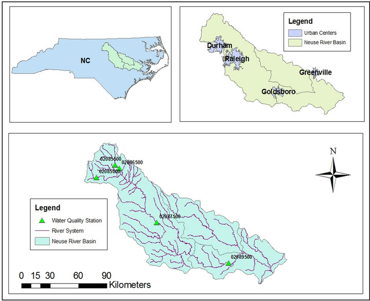
Figure 1. Neuse River Basin in North Carolina, USA with locations of water quality monitoring stations.
user friendly computer program for load estimation developed by the United States Geological Survey (USGS) [16]. It is widely used to estimate nitrogen and phosphorus loads in the rivers [17-21]. The model has been utilized to estimate nutrient flux in the major rivers flowing to the Gulf of Mexico [22] and to calculate “observed” loads in the USGS SPARROW model [23].
Model performance was evaluated using statistical techniques by comparing model-predicted nutrient loads to actual measured loads. How well the regression model predicted nutrient loads to actual measured values is assumed to be indicative of how well the model might be expected to perform for days where no samples were collected. The objectives of this study were to test the performance of a suite of regression models in predicting continuous water quality loading data and to determine systematic bias in the prediction.
2. Materials and Method
2.1. LOADEST Description
The LOADEST was developed by the USGS [16] to estimate constituent loads in streams and rivers through a set of regression models. It needs information on a time series of streamflow, additional data variables and constituent concentrations. The simplest form of linear regression equation consists of log of instantaneous load related with one or more explanatory variables:
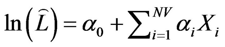 (2)
(2)
where a0 and aj are model coefficients, NV is the number of explanatory variables, and Xj is an explanatory variable. The number and form of explanatory variables is highly dependent on the system under study and the constituent of study. For example, one variable (log of stream flow) was found sufficient for the prediction of suspended sediments [24] whereas a model with six explanatory variables were found suitable for nutrient rating curve [15]. While the estimation method is very straightforward, the process is complicated due to several statistical complications including retransformation bias, data censoring and non-normality of the data. [25] noted that the model bias could lead as much as 50 percent from the true load. LOADEST used three methods to deal with these issues namely maximum likelihood estimation (MLE), adjusted maximum likelihood estimation (AMLE) and least absolute deviation (LAD) methods.
In this study, we used AMLE method [26], the primary load estimation method, which assumes that the model residuals are normally distributed with constant variance. A series of 9 predefined modeling options that vary with number of explanatory variables are provided within the framework of LOADEST. The selection of the predefined model is based on user’s knowledge of the hydrologic and biogeochemical system or alternatively one can use model’s automated method of selection where it selects the “best” model for which the lowest value for Akaike Information Criterion (AIC) and the highest value for Schwarz Posterior Probability Criterion (SPPC) are obtained. Details on other background information on LOADEST can be found in [16].
2.2. Study Area and Data Analysis
This study performed statistical analyses to evaluate historical water quality and flow data collected from various water quality monitoring stations located throughout the Neuse River Basin, North Carolina, USA (Figure 1). It is located in the southeastern part of the country draining an area of over 15,540 km2 into the Atlantic Ocean. A big threat to water quality in the basin are large quantities of nutrients primarily nitrogen and phosphorus, contributed primarily through non-point sources.
Water quality and flow data were obtained for five water quality monitoring stations across the watershed from USGS (www.nwis.waterdata.usgs.gov). A total of seven water quality parameters mainly nitrogen, phosphorus and their variants were collected. Table 1 lists pertinent information on these sites. While total nitrogen (TN) and total phosphorus (TP) has significant amount of monitoring data, others (ammonia, nitrate, nitrite and ortho-phosphate) are limited and not-available in many cases. Data locations were selected in a way that the drainage area could vary for possible correlation analyses with the drainage area and model performance.
The performance of the regression model was evaluated using three statistical evaluations.
1) The partial load factor (PLF) was obtained by dividing long term average estimated data by long-term average measured data. PLF of 1 means the perfect estimation. Less than 1 indicates under prediction while more than 1 indicates over prediction.
2) The Nash-Sutcliffe Efficiency (NSE) coefficient can be defined as:
 (3)
(3)
The value of NSE can range from –∞ to 1. An efficiency of 1 (E = 1) corresponds to a perfect match of modeled discharge to the observed data. An efficiency of 0 (E = 0) indicates that the model predictions are as accurate as the mean of the observed data, whereas an efficiency less than zero (E < 0) occurs when the residual variance is larger than the data variance.
3) The coefficient of determination (R2) describes the degree of collinearity between simulated and measured data. It ranges from 0 to 1, with higher values indicating less error variance, and typically values greater than 0.5 are considered acceptable.
3. Results and Discussion
The collected water quality data from all five stations were tested for outliers and consistency, and finally reformatted as per the requirements of LOADEST. The model was then executed for each parameter individually. Model’s in-built option for automatic selection of predefined regression model using the AIC statistics was chosen in all model executions. The model output related to the AMLE estimation method was selected for analyses.
3.1. LOADEST Prediction
The model output for the average annual loading was compared with the “true” loading which was estimated by calculating instantaneous daily loading (multiplying concentration by daily flow volume) and multiplying the resulting load by 365 days to obtain the annual loading. Table 2 shows the percent difference in loading estimation predicted by LOADEST when compared with the true loading. It clearly indicates that the model over predicted the loading most of the times except for few cases. TN was over predicted by an average of 5% from the true loading on four stations and under predicted the load by 1% at one station. Ammonia and TP were found to be over predicted by 43 and 28% respectively. This is consistent with the outcome of [11,14] where the TP load was found to differ by 30 and 34%.
Model estimated loads were compared with the measured load and statistical indicators PLF, R2 and NSE were calculated. Table 3 lists all statistics for each of the seven parameters for each monitoring locations.
R2 values for TN at all stations varied from 0.97 to 0.99 indicating a very strong correlation between estimated and measured loads. NSE also showed strong correlation with values varied from 0.71 to 0.92. PLF indicated the variation in the range of prediction from −2% to +9% indicating positive bias with mild over prediction.
TP prediction showed similar results as that of TN except for station 02087500 where NSE resulted in −1.76. Negative efficiency indicated a bias in prediction with

Table 1. Monitoring stations and number of samples of water quality constituents in the Neuse River Basin.
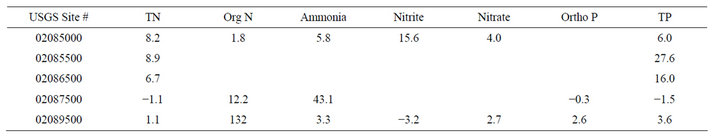
Table 2. Percentage difference between model predicted loading and “true” loading.

Table 3. Sumamry of statistical performance for all water quality parameters.
values accumulated well in one place (higher R2) but far from the 1:1 line of estimated vs. measured comparison. PLF data identified range of prediction from −23% to +28% indicating a balance in bias with a slight over prediction.
Org N estimation showed good correlation with bias toward over prediction that ranged from −1% to +12%. Ammonia was found to be over predicted significantly (43%) and the correlation was very poor to none. Nitrate, nitrite, and ortho-phosphate behaved similarly with good prediction correlation with slight to none over prediction. Figures 2 and 3 are example plots of the best and worst prediction of LOADEST as determined by R2.
Analysis was also extended to examine whether the
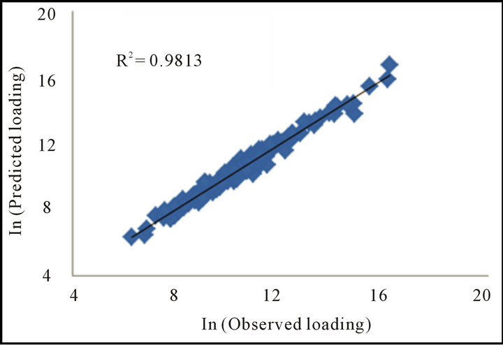
Figure 2. The “best” case of correlation (TN at Eno River, Hillsboro, USGS site # 02085000).

Figure 3. The “worst” case of correlation (Org N at Neuse River near Clayton, USGS Site # 02087500).
sampling size has any impact on the model’s prediction accuracy. While it seemed like there might be a pattern of lower number of sample size causing over prediction, but it was not conclusive. For example, sample size of 77 at site # 02087500 had an average annual loading of 7394 kg/km2 whereas sample size of 294 at site # 02089500 was found to have 3162 kg/km2.
3.2. Time Series Analysis
Time series graphs (Figure 4) were plotted for two parameters, TN and TP, for all five monitoring sites for which complete datasets were available. It facilitated a visual inspection of the model performance and identified possible model bias and trends both in model predictions as well as in observed (or measured) data. As indicated in Figure 4, LOADEST estimated loadings were extrapolated beyond the period for which the measured data were available. It was due to the fact that the flow data were available for longer duration and all was used in the LOADEST estimation.
Load estimation pattern was found different for different simulations (i.e. model executions). This may be due to the fact that each simulation chose a different regression model from a given set of 9 pre-defined models. LOADEST selects best model based on the minimum value of AIC which optimizes between goodness-of-fit and model complexity. For three sites, the model selected the same pre-defined model for both TN and TP but it was different for the other two sites. No conclusive idea could be formed on whether the model selection was adequate. More research is needed in this area.
In general, the prediction and its trend seem to follow the observed data very well. Site-by-site analyses of model prediction are provided in Table 4.
Overall, the LOADEST model was found to perform well in predicting loads. However, a clear understanding of the regression models is needed for better application of the model. Analyzing several regression models provided within the LOADEST environment may provide enough evidence to select the best model for load estimation. Even though the statistical evaluator provides strong correlation, it may be misleading often times, so a visual inspection is necessary which complements the process of selecting the best regression model for the chosen parameter and the study region.
4. Conclusions
Accurate estimation of nutrient loads in the river and
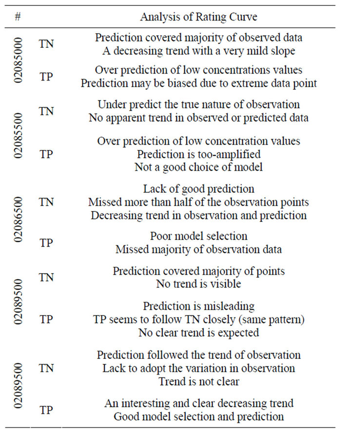
Table 4. Analysis of rating curve.

Figure 4. LOADEST derived rating curve estimation and comparison with the observed data.
streams is very necessary for many applications. There are many methods of load estimation which varies widely from the selection of the model to the ranges of errors it can produce. This study used the LOADEST model which includes several predefined regression models that specify the model form and complexity. Water quality data primarily nitrogen and phosphorus from five monitoring stations in the Neuse River Basin in North Carolina, USA were used in the development and analyses of the rating curves. The AMLE option of the model development was used along with automatic option of selecting pre-defined set of regression models. The performance of the model was evaluated using three statistical indicators: R2, NSE and PLF.
We can conclude that LOADEST performed well in predicting loading in the stream of varying sample sizes and drainage area with bias towards over estimation most of the time. TN was over predicted by an average of 5% from the true loading on five stations and under predicted the load by 1% at one station. Ammonia and TP were found to be over predicted by 43 and 28% respectively. Model performed very well statistically for TN as indicated by R2 range from 0.97 to 0.99, NSE range from 0.71 to 0.92, and PLF range from −2 to 9%. Time series analyses for examining trend of predicted loads produced mixed results with the selection of best models to poor fitting models. But in most cases, model selection did a good job in predicting loads and capturing the trend of observed data.
Even though LOADEST seems to work well in-general and statistics seem to sought a strong correlation in prediction, a clear understanding of the regression model and its selection is important for its application. A timeseries analyses is a must for detecting potential problems with the model selection and identifying possible trends in the observed data as well as in estimated rating curves. It is recommended to test multiple pre-defined regression models before concluding to a final and best model for rating curve development. Future study should also consider filtering observed data and exclude exogenous data from analysis which may potentially affect the model selection process leading to the erroneous prediction.
REFERENCES
- R. B. Alexander, R. A. Smith, G. E. Schwarz, E. W. Boyer, J. V. Nolan and J. W. Brakebill, “Differences in Phosphorous and Nitrogen Delivery to the Gulf of Mexico from the Mississippi River Basin,” Environmental Science & Technology, Vol. 42, No. 3, 2008, pp. 822-830. doi:10.1021/es0716103
- S. D. Preston, V. J. Bierman Jr. and S. E. Sillman, “An Evaluation of Methods for the Estimation of Tributary Mass Loads,” Water Resources Research, Vol. 25, No. 6, 1989, pp. 1379-1389. doi:10.1029/WR025i006p01379
- A. Ullrich and M. Volk, “Influence of Different Nitrate-N Monitoring Strategies on Load Estimation as a Base for Model Calibration and Evaluation,” Environmental Monitoring and Assessment, Vol. 171, No. 1-4, 2010, pp. 513-527. doi:10.1007/s10661-009-1296-8
- M. K. Jha, K. E. Schilling, P. W. Gassman and C. F. Wolter, “Targeting Land-Use Change for Nitrate-Nitrogen Load Reductions in an Agricultural Watershed,” Journal of Soil and Water Conservation, Vol. 65, No. 6, 2010, pp. 342-352. doi:10.2489/jswc.65.6.342
- M. K. Jha, C. F. Wolter, P. W. Gassman and K. E. Schilling, “Assessment of TMDL Implementation Strategies for Nitrate Impairment of the Raccoon River, Iowa,” Journal of Environmental Quality, Vol. 39, No. 4, 2010, pp. 1317-1327. doi:10.2134/jeq2009.0392
- M. K. Jha, J. G. Arnold and P. W. Gassman, “Water Quality Modeling for the Raccoon River Watershed Using SWAT,” Transactions of the ASABE, Vol. 50, No. 2, 2007, pp. 479-493.
- I. G. Littlewood, C. D. Watts and J. M. Custance, “Systematic Application of United Kingdom River Flow and Quality Databases for Estimating Annual River Mass Loads (1975-1994),” Science of the Total Environment, Vol. 210-211, 1998, pp. 21-40. doi:10.1016/S0048-9697(98)00042-4
- K. E. Schilling and Y. K. Zhang, “Baseflow Contribution to Nitrate-Nitrogen Export from a Large Agricultural Watershed USA,” Journal of Hydrology, Vol. 295, No. 1-4, 2004, pp. 305-316. doi:10.1016/j.jhydrol.2004.03.010
- Y. Guo, M. Markus and M. Demissie, “Uncertainty of Nitrate-N Load Computations for Agricultural Watersheds,” Water Resources Research, Vol. 38, No. 10, 2002, p. 1185. doi:10.1029/2001WR001149
- B.T. Aulenbach and R. P. Hooper, “The Composite Method: An Improved Method for Stream-Water Solute Load Estimation,” Hydrological Processes, Vol. 20, No. 14, 2006, pp. 3029-3047. doi:10.1002/hyp.6147
- F. Moatar and M. Meybeck, “Compared Performance of Different Algorithms for Estimating Annual Nutrient Loads Discharged by the Eutrophic River Loire,” Hydrological Processes, Vol. 19, No. 2, 2005, pp. 429-444. doi:10.1002/hyp.5541
- Z. Li, Y. K. Zhang, K. Schilling and M. Skopec, “Cokriging Estimation of Suspended Sediment Loads,” Journal of Hydrology, Vol. 327, No. 3-4, 2006, pp. 389-398. doi:10.1016/j.jhydrol.2005.11.028
- A. Zamyadi, J. Gallichand and M. Duchemin, “Comparison of Methods for Estimating Sediment and Nitrogen Loads from a Small Agricultural Watershed,” Canadian Society of Bioengineering, Vol. 49, 1-2, 2007, pp. 127- 136.
- D. M. Robertson and E. D. Roerish, “Influence of Various Water Quality Sampling Strategies on Load Estimates for Small Streams,” Water Resources Research, Vol. 35, No. 12, 1999, pp. 3747-3759. doi:10.1029/1999WR900277
- T. A. Cohn, D. L. Caulder, E. J. Gilroy, L. D. Zynjuk and R. M. Summers, “The Validity of a Simple Statistical Model for Estimating Fluvial Constituent Loads: An Empirical Study Involving Nutrient Loads in Chesapeake Bay,” Water Resources Research, Vol. 28, No. 9, 1992, pp. 2353-2363. doi:10.1029/92WR01008
- USGS LOADEST, “Load Estimator (LOADEST): A Fortran Program for Estimating Constituent Loads in Streams and Rivers. Techniques and Models Book 4,” Chapter 5, US Geological Survey, Reston, 2004.
- D. A. Goolsby, W. A. Battaglin, B. T. Aulenbach and H. P. Hooper, “Nitrogen Flux and Sources in the Mississippi River Basin,” Science of the Total Environment, Vol. 248, No. 2-3, 2000, pp. 75-86. doi:10.1016/S0048-9697(99)00532-X
- D. A. Goolsby and W. A. Battaglin, “Long-Term Changes in Concentrations and Flux of Nitrogen in the Mississippi River Basin, USA,” Hydrological Processes, Vol. 15, No. 7, 2001, pp. 1209-1226. doi:10.1002/hyp.210
- R. P. Hooper, B. T. Aulenbach, and V. J. Kelly, “The National Stream Quality Accounting Network: A FluxBased Approach to Monitoring the Water Quality of Large Rivers,” Hydrological Processes, Vol. 15, No. 7, 2001, pp. 1089-1106. doi:10.1002/hyp.205
- B. T. Aulenbach and R. P. Hooper, “The Composite Method: An Improved Method for Stream-Water Solute Load Estimation,” Hydrological Processes, Vol. 20, No. 14, 2006, pp. 3029-3047. doi:10.1002/hyp.6147
- T. R. Maret, D. E. MacCoy and D. M. Carlisle, “LongTerm Water Quality and Biological Responses to Multiple Best Management Practices in Rock Creek, Idaho,” Journal of the American Water Resources Association, Vol. 44, No. 5, 2008, pp. 1248-1269. doi:10.1111/j.1752-1688.2008.00221.x
- USGS, “USGS Open-File Report 2007-1080—Streamflow and Nutrient Fluxes of the Mississippi-Atchafalaya River Basin and Subbasins for the Period of Record through 2005, Methods Used to Estimate Nutrient Fluxes,” 2009. http://toxics.usgs.gov/pubs/of-2007-1080/methods.html
- USGS, “Application of Spatially Referenced Regression Modeling for the Evaluation of Total Nitrogen Loading in the Chesapeake Bay Watershed,” 2009. http://md.water.usgs.gov/publications/wrir-99-4054/html/index.htm
- C. G. Crawford, “Estimation of Suspended-Sediment Rating Curves and Mean Suspended Sediment Loads,” Journal of Hydrology, Vol. 129, No. 1-4, 1991, pp. 331-348. doi:10.1016/0022-1694(91)90057-O
- R. I. Ferguson, “River Loads Underestimated by Rating Curves,” Water Resources Research, Vol. 22, No. 1, 1986, pp. 74-76. doi:10.1029/WR022i001p00074
- USGS, “Statistical Methods in Water Resources,” In: D. R. Helsel and R. M. Hirsch, Eds., Techniques of WaterResources Investigations, US Geological Survey, 2002, p. 522. http://water.usgs.gov/pubs/twri/twri4a3
NOTES
*Corresponding author.