ABSTRACT

In this paper an inventory model is developed with time dependent power pattern demand and shortages due to deterioration and demand. The deterioration is assumed to follow a two parameter Weibull distribution. Three different cases with complete, partial, no backlogging are considered. The optimal analytical solution of the model is derived. Suitable numerical example has been discussed to understand the problem. Further sensitivity analysis of the decision variables has been done to examine the effect of changes in the values of the parameters on the optimal inventory policy.

1. Introduction

Deterioration of items in an inventory is a common phenomenon in business situations. This is due to the fact that the items in the inventory become obsolete, devalued, decay or damaged depending on the type of goods. As a consequence of the deterioration shortages may occur. Hence deterioration factor has to be given importance while determining the optimal policy for an inventory model.

Whitin [1] was the first to consider the deterioration of inventory items, he dealt with the deterioration of fashion goods at the end of prescribed storage period. Ghare and Schrader [2] later formulated a mathematical model with a constant deterioration rate. Covert and Philip [3] then extended Ghare and Schrader’s model for variable rate of deterioration by assuming two parameter Weibull distribution functions.

Resently, researchers are analyzing the effect of deterioration and the variations in the demand rate with time in supply chain and logistics. Dave and Patel [4] derived a lot size model for constant deterioration of items with time proportional demand. Sachan [5] modified Dave and Patel’s [4] model. Goel and Aggarwal [6] formulated an order-level inventory system with power-demand pattern for deteriorating items. Datta and Pal [7] presented an EOQ model with the demand rate dependent on instantaneous stock displayed until a predefined maximum level of inventory L is achieved. After this level is reached, the demand rate becomes constant (D(t) = a[I(t)^b] for I(t) > L and D(t) = aL^b for 0 £ I(t) £ L). Chang and Dye [8] developed an EOQ model with a similar power demand and considered partial backlogging of orders. He stated that if longer the waiting time smaller the backlogging rate would be. So the proportion of the customers who would like to accept backlogging at time t decreases with the waiting time for the next replenishment. In this situation the backlogging rate is defined as

(1.1)

where t_i is the time at which the i^th replenishment is being made and δ is the backlogging parameter. Several researchers have extended their idea to different situations considering various deterioration rates and time value of money. Valuable models in this direction are the models of S. R. Singh, and T. J. Singh [9], Tarun Jeet Singh, Shiv Raj Singh and Rajul Dutt [10], C. K. Tripathy and L. M. Pradhan [11], etc.

In continuation with these developments an inventory model for Weibull deteriorating items is developed in this paper with power pattern time dependent demand. Shortages are allowed with backlogging of orders. An analytical solution of the mode is derived and illustrated with the help of numerical examples. The sensitivity analysis of the optimal solution is carried out with respect to changes in various parametric values. These changes are depicted in the Tables 1-3 in Section 4.

2. Notations and Assumptions

2.1. Notations

A: The ordering cost per inventory cycle.

C: The purchase cost per unit.

H: The inventory holding cost per unit per time unit.

p_b: The backordered cost per unit short per time unit.

p_l: The cost of lost sales per unit.

t₁: The time at which the inventory level reaches zero, t₁ ³ 0.

t₂: The length of period during which shortages are allowed, t₂ ³ 0.

T: (= t₁ + t₂) The length of cycle time.

I_m: The maximum inventory level during [0, T].

I_b: The maximum backordered units during stock out period.

Q_i: (= I_m + I_b) The order quantity in cycle of length T corresponding to no backlogging, partial backlogging and complete backlogging).

I₁(t): The level of positive inventory at time t, 0 £ t £ t₁.

I₂(t): The level of negative inventory at time t, t₁ £ t £ T.

K_i: The total cost per time unit.

• 2.2. Assumptions

• The inventory consists of only one type of items.

• The expression for demand rate is at any time t, where d is a positive constant, n may be any positive number, T is the planning horizon.

• The variable deterioration rate q(t) is assumed to follow the two parameter weibull distribution function (i.e.) q(t) = αβt^β-1, where α is the scale parameter, α > 0; β is the shape parameter β > 0; t is the time to deterioration, t > 0. The replenishment rate is infinite.

• The lead-time is zero or negligible.

• The planning horizon is infinite.

• During the stock out period, the backlogging rate is variable and is dependent on the length of the waiting time for the next replenishment. The proportion of the customers who would like to accept the backlogging at time “t” is with the waiting time (T - t) for the next replenishment i.e., for the negative inventory the backlogging rate is; d > 0 denotes the backlogging parameter and t₁ £ t £ T.

3. Mathematical Model

With above assumptions, the on-hand inventory level at any instant of time is exhibited in Figure 1.

3.1. Inventory Level before Shortage Period

During the period [0, t₁], the inventory depletes due to the demand and deterioration. Hence, the differential equation governing the inventory level I₁(t) at any time t during the cycle [0, t₁] is given by

(3.1)

with the boundary condition I₁(t₁) = 0 at t = t₁.

The solution of Equation (3.1) is given by

(3.2)

The maximum positive inventory level is

(3.3)

3.1.1. Model I: (No Backlogging)

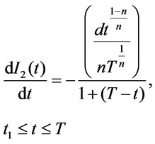
The state of inventory during the shortage period [t₁,T] is represented by the differential equation,

(3.4)

with the boundary condition I₂(t₁) = 0 at t = t₁.

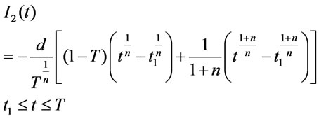
The solution of Equation (3.4) is given by

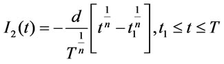(3.5)

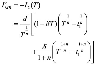
The maximum backordered units are

(3.6)

Hence, the order size during [0,T] is Q₁ = I_MI + I_MB.

(3.7)

3.1.1.1. Cost Components The total cost per replenishment cycle consists of the following cost components.

3.1.1.2. Ordering Cost per Cycle (I_OC)

(3.8)

3.1.1.3. Inventory Holding Cost per Cycle (I_HC)

(3.9)

3.1.1.4. Backordered Cost per Cycle (I_BC)

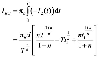(3.10)

3.1.1.5. Purchase Cost per Cycle (I_PC)

(3.11)

Hence, the total cost per time unit from (3.8), (3.9), (3.10), (3.11) is

(3.12)

To minimize total average cost per unit time (K₁), the optimal value of t₁ can be obtained by solving the equation

(3.13)

The value of t₁ obtained from (3.13) is used to obtain the optimal values of Q₁ and K₁. Since the Equation (3.13) is nonlinear, it is solved using MATLAB.

The condition, is also satisfied for the value t₁ from (3.13).                                 (3.14)

3.1.2. Model II: (Partial Backlogging)

3.1.2.1. Inventory Level during Shortage Period During the interval [t₁,T] stock out situation arises. The orders during this period are partially backlogged. The state of inventory during [t₁,T] can be represented by the differential equation,

(3.15)

with the boundary condition I₂(t₁) = 0 at t = t₁.

The solution of Equation (3.4) is given by

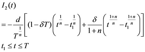(3.16)

The maximum backordered units are

(3.17)

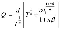
Hence, the order size during [0,T] is.

(3.18)

3.1.2.2. Cost Components The total cost per replenishment cycle consists of the following cost components.

3.1.2.3. Backordered Cost per Cycle ()

(3.19)

3.1.2.4. Cost Due to Lost Sales per Cycle (I_LS)

(3.20)

3.1.2.5. Purchase Cost per Cycle ()

(3.21)

Hence, the total cost per time unit from (3.8), (3.9), (3.19), (3.20), (3.21) is

(3.22)

To minimize total average cost per unit time (K₂), the optimal value of t₁ can be obtained by solving the equation

(3.23)

The value of t₁ obtained from (3.23) is used to obtain the optimal values of Q₂ and K₂. Since the Equation (3.23) is nonlinear, it is solved using MATLAB.

The condition, is also satisfied for the value t₁ from (3.23).                                 (3.24)

3.1.3. Model III: (Complete Backlogging)

3.1.3.1. Inventory Level during Shortage Period During the interval [t₁,T] stock out situation arises. the orders during this period are completely backlogged. The state of inventory during [t₁,T] can be represented by the differential equation,

(3.25)

with the boundary condition I₂(t₁) = 0 at t = t₁.

The solution of Equation (3.4) is given by

(3.26)

The maximum backordered units are

(3.27)

Hence, the order size during [0,T] is.

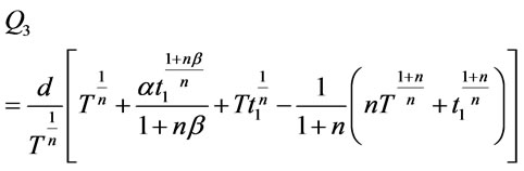(3.28)

3.1.3.2. Cost Components The total cost per replenishment cycle consists of the following cost components.

3.1.3.3. Backordered Cost per Cycle ()

(3.29)

3.1.3.4. Cost Due to Lost Sales per Cycle ()

(3.30)

3.1.3.5. Purchase Cost per Cycle ()

(3.31)

Hence, the total cost per time unit from (3.8), (3.9), (3.29), (3.30), (3.31) is

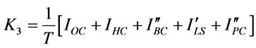(3.32)

To minimize total average cost per unit time (K₃), the optimal value of t₁ can be obtained by solving the equation

(3.33)

The value of t₁ obtained from (3.33) is used to obtain the optimal values of Q₃ and K₃. Since the Equation (3.33) is nonlinear, it is solved using MATLAB.

The condition, is also satisfied for the value t₁ from (3.33).                                   (3.34)

To illustrate and validate the proposed model, appropriate numerical data is considered and the optimal values are found in the following section. Sensitivity analysis is carried out with respect to backlogging parameter and deterioration rate.

4. Numerical Example and Sensitivity Analysis

In this section the optimal value (), the optimal order quantity () and the minimum total average cost () are computed for the data given below:

d = 50 units, n = 2 units, T = 1 year, A = $ 250 per order, C = $ 8.0 per unit, h = $ 0.50 per unit per year, p_b = $ 12.0 per unit per year, p_l= $ 15.0 per unit, d =0.04 units, α = 0.01, b = 4.

4.1. Optimum Solution

4.1.1. Model I

For the above numerical values, when deterioration rate is 5%, the optimum time t₁ at which positive inventory is zero is 0.489604 time units and stock out period t₂ is of length is 0.510396 time units. This advices the retailer to buy 50 units which will cost a minimum of $ 770.06 (by rounding off).

The following observations have been made on the basis of the above table with the increase in scale parameter (α) and shape parameter (β):

• Increase in α results in decrease in inventory period, increase in order quantity and increase in total cost per time unit.

• Increase in β results in increase in inventory period, decrease in order quantity and decrease in total cost per time unit.

Hence in general 50% change in the parameters α, β results only in a marginal change in total cost per time unit.

4.1.2. Model II

For the above numerical values, when deterioration rate is 5%, the optimum time t₁ at which positive inventory is zero is 0.962174 time units and stock out period t₂ is of length is 0.037826 time units. This advices the retailer to buy 50 units which will cost a minimum of $ 658.20 (by rounding off Q_i^*).

The following observations have been made on the basis of the above table with the increase in backlogging parameter, scale parameter and shape parameter:

• Increase in δ results in increase in inventory period, decrease in order quantity and increase in total cost per time unit.

• Increase in α results in decrease in inventory period, increase in order quantity and increase in total cost per time unit.

• Increase in β results in increase in inventory period, decrease in order quantity and decrease in total cost per time unit.

Hence in general 50% change in the parameters δ, α, β results only in a marginal change in total cost per time unit.

4.1.3. Model III

For the above numerical values, when deterioration rate is 5%, the optimum time t₁ at which positive inventory is zero is 0.969997 time units and stock out period t₂ is of length is 0.030003 time units. This advices the retailer to buy 50 units which will cost a minimum of $ 658.28 (by rounding off).

The following observations have been made on the basis of the above table with the increase in scale parameter and shape parameter:

• Increase in α results in decrease in inventory period, increase in order quantity and increase in total cost per time unit.

• Increase in β results in increase in inventory period, decrease in order quantity and decrease in total cost per time unit.

Hence in general 50% change in the parameters α, β results only in a marginal change in total cost per time unit.

5. Conclusion

In this paper, we have developed a deterministic inventtory model with power pattern demand and Weibull deterioration rate. This type of power pattern demand requires a different policy based on general Weibull pattern. In cases when large portion of demand occurs at the beginning of the period n > 1 will be used and when it is large at the end 0 < n < 1 is used. Similarly n = 1 and n = ∞ correspond to constant demand and instantaneous demand respectively. Focusing on this concept the optimal order quantity has been computed, for three different cases namely, no backlogging, partial backlogging and complete backlogging, by minimizing the total inventory cost and the minimized objective cost function is observed to be strictly convex. Sensitivity analysis has been carried out with the change in parameters. The total cost is seen to decrease with backlogging of orders.

REFERENCES

- G. Hadley and T. M. Whitin, “Analysis of Inventory Systems,” Prentice-Hall, New Jersey, 1963.
- P. M. Ghare and G. F. Schrader, “A Model for an Exponentially Decaying Inventory,” Journal of Industrial Engineering, Vol. 14, 1963, pp. 238-243.
- R. P. Covert and G. C. Philip, “An EOQ Model for Deteriorating Items with Weibull Distributions Deterioration,” AIIE Transactions, Vol. 5, No. 4, 1973, pp. 323-332. doi:10.1080/05695557308974918
- U. Dave and L. K. Patel, “(T, Si) Policy Inventory Model for Deteriorating Items with Time Proportional Demand,” Journal of the Operational Research Society, Vol. 32, 1981, pp. 137-142.
- R. S. Sachan, “On (T, Si) Policy Inventory Model for Deteriorating Items with Time Proportional Demand,” Journal of the Operational Research Society, Vol. 35, No. 11, 1984, pp. 1013-1019.
- V. P. Goel and S. P. Aggarwal, “Order Level Inventory System with Power Demand Pattern for Deteriorating Items,” Proceedings of the All India Seminar on Operational Research and Decision Making, University of Delhi, New Delhi, 1981, pp. 19-34.
- T. K. Datta and A. K. Pal, “Order Level Inventory System with Power Demand Pattern for Items with Variable Rate of Deterioration,” Indian Journal of Pure and Applied Mathematics, Vol. 19, No. 11, 1988, pp. 1043-1053.
- H. J. Chang and C. Y. Dye, “An EOQ Model for Deteriorating Items with Time Varying Demand and Partial Backlogging,” Journal of the Operational Research Society, Vol. 50, No. 11, 1999, pp. 1176-1182.
- S. R. Singh and T. J. Singh, “An EOQ Inventory Model with Weibull Distribution Deterioration, Ramp Type Demand and Partial Backlogging,” Indian Journal of Mathematics and Mathematical Sciences, Vol. 3, No. 2, 2007, pp. 127-137.
- T. J. Singh, S. R. Singh and R. Dutt, “An EOQ Model for Perishable Items with Power Demand and Partial Backlogging,” International Journal of Production Economics, Vol. 15, No. 1, 2009, pp. 65-72.
- C. K. Tripathy and L. M. Pradhan, “An EOQ Model for Weibull Deteriorating Items with Power Demand and Partial Backlogging,” International Journal of Contemporary Mathematical Sciences, Vol. 5, No. 38, 2010, pp. 1895-1904.