Applied Mathematics
Vol. 4 No. 5 (2013) , Article ID: 31471 , 8 pages DOI:10.4236/am.2013.45112
Symbolic and Graphical Computations of a Class of Slightly Perturbed Equations
1Department of Astronomy, Faculty of Science, King Abdulaziz University, Jeddah, Saudi Arabia
2Department of Astronomy, National Research Institute of Astronomy and Geophysics, Cairo, Egypt
3Department of Mathematics, College of Science for Girls, King Abdulaziz University, Jeddah, Saudi Arabia
Email: Sharaf_adel@hotmail.com, *Saad6511@gmail.com, Zammomin@hotmail.com
Copyright © 2013 Mohammed A. Sharaf et al. This is an open access article distributed under the Creative Commons Attribution License, which permits unrestricted use, distribution, and reproduction in any medium, provided the original work is properly cited.
Received March 14, 2013; revised April 14, 2013; accepted April 21, 2013
Keywords: Symbolic Computation; Small Perturbations; Graphical Representations; Transcendental Equations
ABSTRACT
In this paper, a class of slightly perturbed equations of the form  will be treated graphically and symbolically, where
  is an analytic function of x. For graphical developments, we set up a simple graphical method for the real roots of the equation
  illustrated by four transcendental equations. In fact, the graphical solution usually provides excellent initial conditions for the iterative solution of the equation. A property avoiding the critical situations between divergent to very slow convergent solutions may exist in the iterative methods in which no good initial condition close to the root is available. For the analytical developments, literal analytical solutions are obtained for the most celebrated slightly perturbed equation which is Kepler’s equation of elliptic orbit. Moreover, the effect of the orbital eccentricity on the rate of convergence of the series is illustrated graphically.
1. Introduction
Symbolic Computation is a modern area of research of interdisciplinary character that is placed in the common area of action of mathematics and the sciences of computation. Symbolic computing is concerned with the representation and manipulation of information in a symbolic form. It is based on defining objects not as numerical quantities but as entities that have certain mathematical properties. The representation of mathematical objects in a symbolic rather than numeric computational form has existed since the early days of computer science [1]. The 1970s and 1980s have seen the development, however, of environments that place a greater emphasis on computation with mathematical objects in an implicit or symbolic form. A brief history of symbolic mathematical computation is given in [2] and references therein.
Symbolic and graphical computations utilized with nowadays existing symbols used for manipulating digital computer programs, they are definitely invaluable for obtaining solutions with any desired accuracy [3,4].
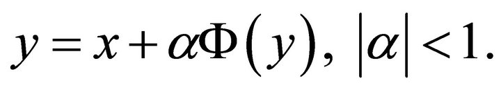
In the present paper, a class of slightly perturbed equations of the form
 , (1)
, (1)
will be treated graphically and symbolically where  is an analytic function of x.
Advances in graphical technology have now made it possible to interact with information in innovative ways, most notably by exploring multimedia environments and by manipulating three-dimensional virtual worlds. In many situations, the graph offers much more insight into the problem than does the algebra. Moreover it makes easy to understand and interpret data at a glance and helps to make comparisons among many things. For the iterative solution of equations, graphical solution usually provides excellent initial conditions.
The above mentioned advantages motivated us introducing graphical and symbolic developments to a class of slightly perturbed equations that would have some applications in the future.
2. Graphical Computations
In this section, simple graphical method for the real roots of the equation
 , (2)
, (2)
will be developed, where ![]() and
and ![]() are given and x is required.
are given and x is required.
Take a rectangular system of axes and construct the curve and the straight line whose equations are
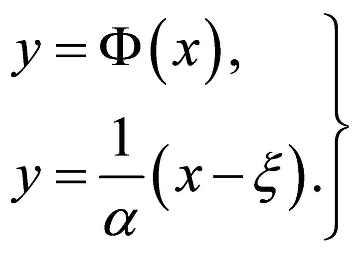 (3)
(3)
The abscissa of their point of intersection is the value of x satisfying the equation; for, eliminating y, Equation results (1). Instead of drawing the straight line a straightedge can be drawn between the two points  and
and , with
  (say).
The accuracy of the computed root (or roots)  may checked by the condition that
 , where
 ![]() is of order 10−3 to 10−1 at most.
is of order 10−3 to 10−1 at most.
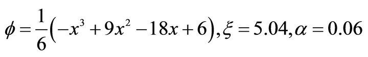
The following are two sets of examples, for the first set we considered four equations listed together with the values of ![]() and
and  in Table 1. While the second set of examples is four cases of the most celebrated slightly perturbed equation which is Kepler’s equation of elliptic orbit given as
 (4)
(4)
where
 (5)
(5)
The angle M, called the mean anomaly by Kepler, E the eccentric anomaly, e the eccentricity of the orbit ,
,  the gravitational parameter, n the mean motion, a the semi-major axis of the orbit, t the time, and
 ![]() is the time of passage through pericenter (the closet point to the focus of the orbit). The solution of Kepler’s equation is to find E when M and e are given.
is the time of passage through pericenter (the closet point to the focus of the orbit). The solution of Kepler’s equation is to find E when M and e are given.
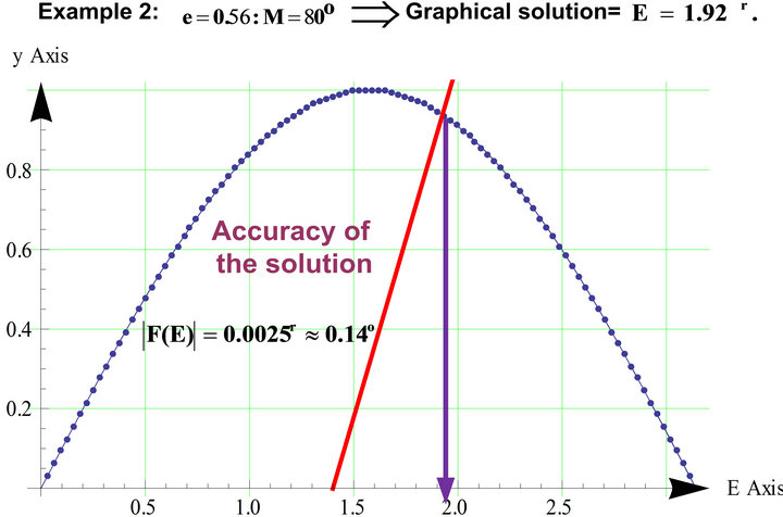
The four cases of Kepler’s equation are listed in Table 2.
Figures 1 and 2 give the solutions of the two sets of equations mentioned in Tables 1 and 2 respectively.
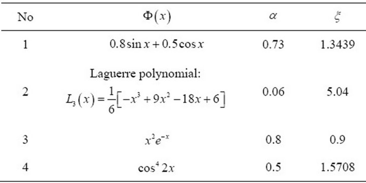
Table 1. Equation (2) for some![]() ,
, ![]() and
and .
.
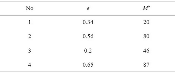
Table 2. Kepler’s equation for some e and M.
3. Symbolic Computations
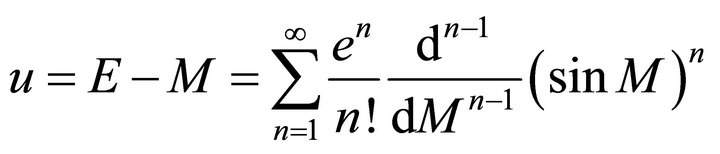
Lagrange’s approach to solving Kepler’s equation in 1770s, led to useful expansion of the Equation (1) as
where ![]() is to be considered a small parameter-originally identified with a planetary eccentricity. Then y could be expanded in terms of x and
is to be considered a small parameter-originally identified with a planetary eccentricity. Then y could be expanded in terms of x and ![]() [5] as
[5] as
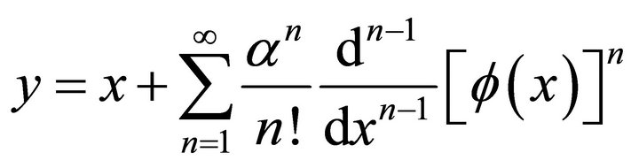 . (6)
. (6)
Lagrange’s series is, of course, the Taylor series representation of the root of the functional equation 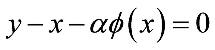 . Sufficient conditions for a unique root are obtained by a direct application of Rouche’s theorem for analytical function of a complex variable [6].
In what follows we shall illustrate the symbolic computations by considering the applications of Equation (6) on the two sets of equations mentioned in Section 2.
3.1. Symbolic Computations of the First Set of Table 1
Because of space limitations, only three terms for the symbolic expressions of the functions of Table 1 are given without specification of the values of ![]() and
and .
.
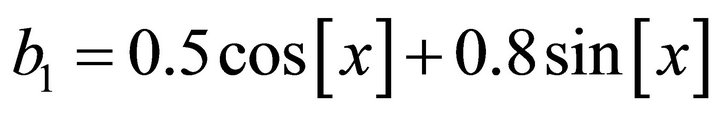
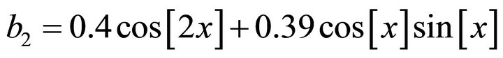
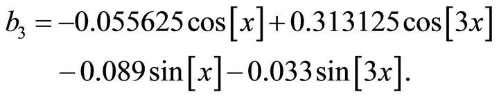
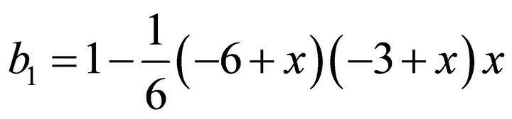
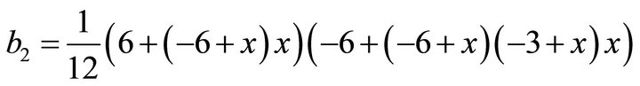
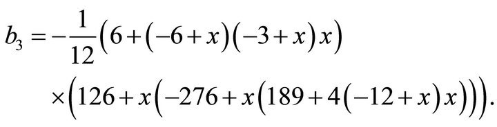
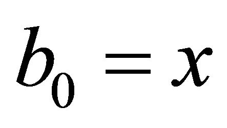
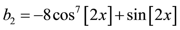
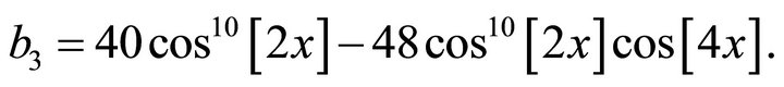
We can write each of these expansions as a third degree polynomial in ![]() as
as
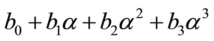
The b’s coefficients are listed in for each function. In what followsFor the function: 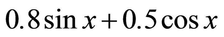

For the Laguerre polynomial L3(x)
 (a)
(a)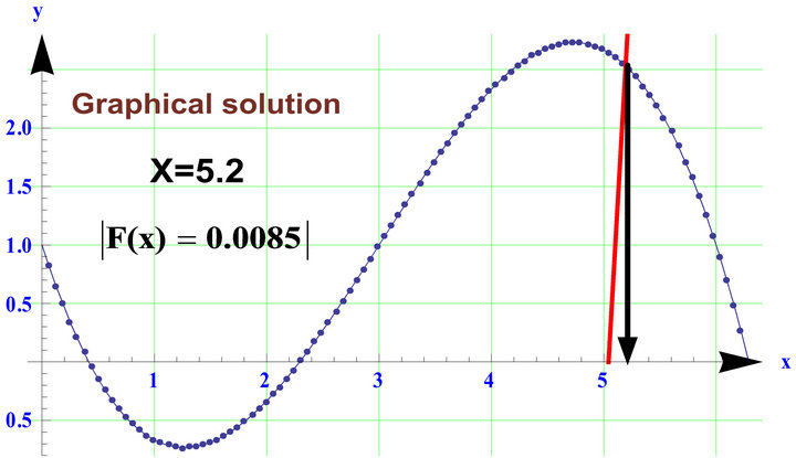 (b)
(b)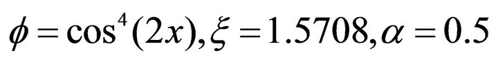 (c)
(c)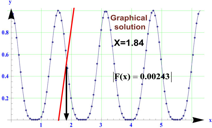 (d)
(d)
For the function 

For the function 

3.2. Symbolic Computations for Kepler’s Equation of Table 2
Comparing Equation (1) with Equation (4) we get:
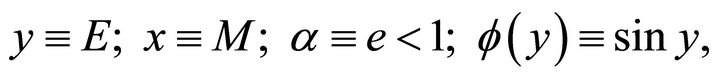
then applying Lagrange’s expansion theorem as given by Equation (5) we obtain:
 , (6)
, (6)
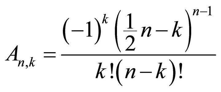
it could be shown that [6],
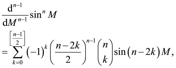 (7)
(7)
 (a)
(a)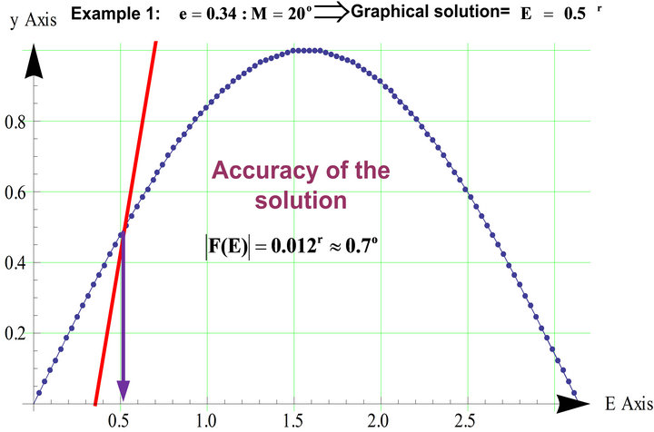 (b)
(b)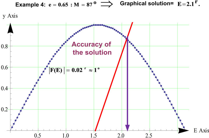 (c)
(c)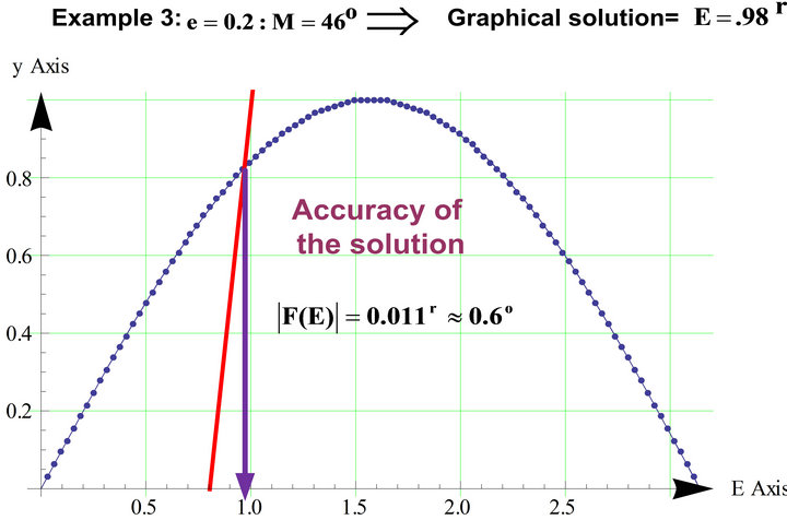 (d)
(d)where [z] is the integer part of z. Using Equation (7) into Equation (6) we get:
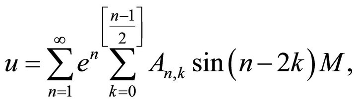 (8)
(8)
where
 . (9)
. (9)
Equation (8) gives the solution of Kepler’s equation as power series in the eccentricity e with the coefficient which turned out to be linear combinations of sine functions of integer multiples of the mean anomaly M. It was shown [5] that  is the requirement for the series (8) to represent the unique root of Kepler’s equation for all values of M. Laplace is the first to show that if e exceeds this critical value, then the series will diverge for some values of M.
Lagrange rearrange the terms in the series (8) to obtain a form which we would now call a Fourier sine series. The Fourier coefficients were infinite power series in e which converge for all elliptic orbits. This series could be written as:
 (10)
(10)
where
 (11)
(11)
 the Bessel function of the first kind of order n.
In 1824, Bessel, attempted the direct solution of Kepler’s equation as a Fourier series and obtained the coefficients in an integral forms. The power series expansions of these integrals produced, of course, the same collection of series that Lagrange had obtained [Equation (10)] almost fifty years earlier-but, because Bessel made such an extensive study of these functions for many years, they bear his name not of Lagrange.
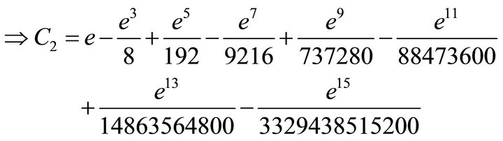
From the above discussions we can write u in the compact form
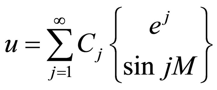 . (12)
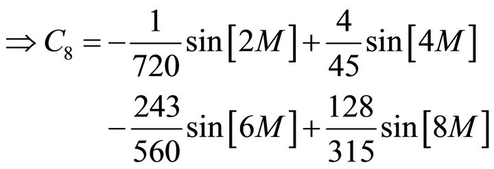
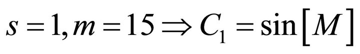
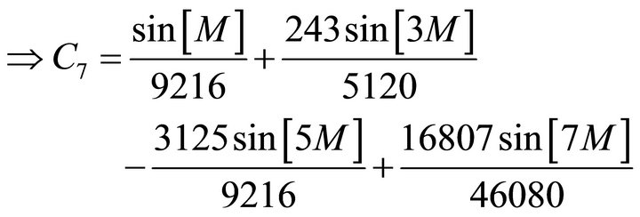
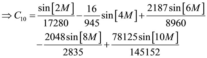
Of course, the analytical expression of any of the C's coefficients is computed from the truncated series of Equation (12).
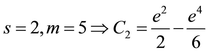
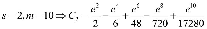
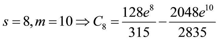
In what follows, we shall find the analytical expression for the coefficient  o
o or of
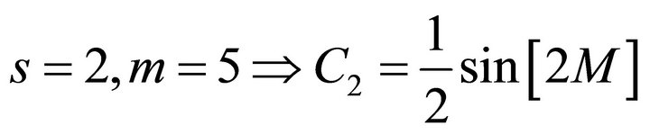
or of  for the series solution of Kepler’s equation for elliptic orbits represented by m terms. To do so, let m (integer) the maximum number of terms for the series solution of Kepler’s equation and s (integer)
  is number of the required term of the series.
3.2.1. Series Solution of the Kepler’s Equation in the Form: 
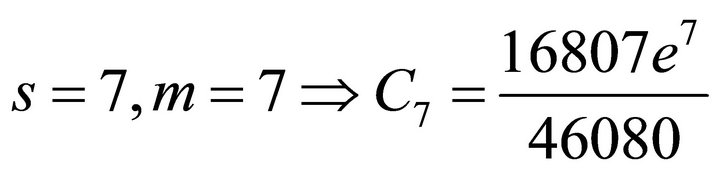

3.2.2. Series Solution of the Kepler’s Equation in the Form: 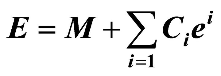
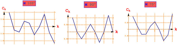
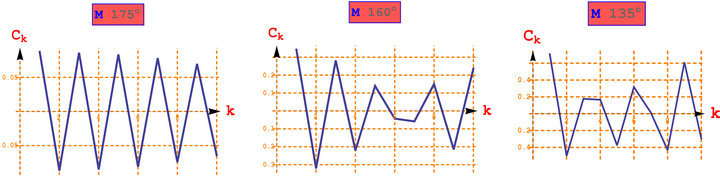
3.3. Graphical Representations of the C's’ Coefficients
First: If  are the coefficients of
In appendix some graphics showing the effect of the eccentricity e on the coefficients, that is, the effect of e on the convergence rate of the series.
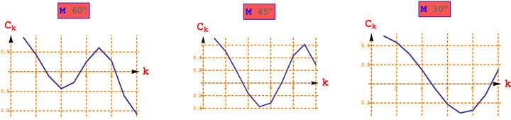
Second: If  are the coefficients of
Graphical representations of the C's coefficients  are also given in appendix.
4. Conclusion
In this paper, symbolic and graphical computation methods are developed for the real roots of the equation 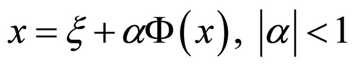 for a class of slightly perturbed equations. Figures 1(a)-(d) show the graphical representations of the transcendental equations given in Table 1. The literal analytical solution of Kepler’s equation of elliptic orbit is described by setting up simple graphical representations. The four cases of slightly perturbed equation (Kepler’s equation) listed in Table 2 are shown by Figures 2(a)-(d). While the graphical representations of the C's coefficients
  and
and ,
,  are given by Figures 3 and 4 in the Appendix. The effect of the orbital eccentricity on the rate of convergence of the series is illustrated graphically. One merit for applying graphical solution is providing excellent initial conditions for iterative solutions of equations.
REFERENCES
- E. Fiume, “An Introduction to Scientific, Symbolic, and Graphical Computation,” A K Peters/CRC Press, London, 1995.
- E. Kaltofen, “Challenges of Symbolic Computation,” Journal of Symbolic Computation, Vol. 29, 2000, pp. 891-919. doi:10.1006/jsco.2000.0370
- V. A. Brumberg, “Analytical Techniques of Celestial Mechanics,” Springer-Verlag, Berlin, Heidelberg, 1995. doi:10.1007/978-3-642-79454-4
- M. A. Sharaf, A.-N. S. Saad and A. A. Sharaf, “Unified Symbolic Algorithm of Gauss Method for Near-Parabolic Orbits,” Celestial Mechanics and Dynamical Astronomy, Vol. 70, No. 3, 1998, pp. 201-214. doi:10.1023/A:1008339612666
- M. P. Fitzpatrick, “Principles of Celestial Mechanics,” Academic Press, New York and London, 1970.
- R. H. Battin, “An Introduction to the Mathematics and Methods of Astrodynamics,” AIAA, Education Series, Reston, 1999. doi:10.2514/4.861543
Appendix
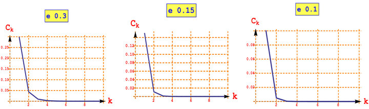
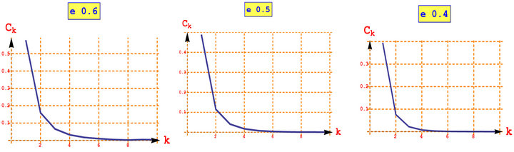
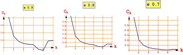
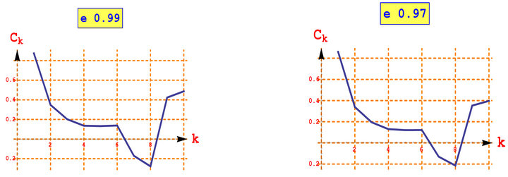
Figure 3. Graphical representations of the C's coefficients![]() . Note that, the series diverge for e ≥ 0.7 as proved by Laplace.
. Note that, the series diverge for e ≥ 0.7 as proved by Laplace.
NOTES
*Corresponding author. Current address: Department of Mathematics, Qassim University, P. O. Box 6595, Buraidah 51452, Saudi Arabia.