Journal of Mathematical Finance
Vol.2 No.1(2012), Article ID:17601,6 pages DOI:10.4236/jmf.2012.21011
From Normal vs Skew-Normal Portfolios: FSD and SSD Rules
School of Economics, University of Rome Tor Vergata, Rome, Italy
Email: sergio.scarlatti@uniroma2.it
Received September 26, 2011; revised November 16, 2011; accepted November 25, 2011
Keywords: Normal Distribution; Skew-Normal Distribution; Mixture Distributions; Stochastic Ordering; Stochastic Dominance; Portfolio Selection; Derivatives; Straddles
ABSTRACT
In this paper we study stochastic dominance rules of first and second order for univariate skew-normal random variables, the analysis being relevant in connection with the problem of portfolio choice in stock markets showing departure from the classical assumption of normality on returns. Besides that, our analysis is also relevant for markets where stocks returns are normally distributed: if standard derivatives are tradable and straddles, characterized by V-shaped pay-outs, are implementable at specific strike prices, then, portfolios including them, can exhibit exact skew-normality in their returns. We provide a set of simple conditions on the statistical parameters of the distributions which imply FSD and SSD and discuss some application of our criteria.
1. Introduction
Ranking portfolio return distributions is one of the key procedures which can be used by quantitative analysts to provide support to the decisional processes of portfolio managers. In this paper we discuss ranking criteria for skew-normal distributions based on stochastic dominance rules of first and second order; we refer the reader to Levy ([1]) for a detailed exposition of these concepts and many related results.
The economical motivation underpinning second order stochastic dominance (SSD) is particularly appealing: a representative investor with increasing and concave utility function will always prefer a portfolio  to a portfolio
  if the the returns of
  stochastically dominate at the second order the returns of
 . SSD encapsulates therefore the concept of risk-aversion. Investments theorists and practitioners have developed along the times several methods to compare risky investments prospects or portfolios of assets and choose among the feasible ones in some optimal way: the review paper Brandt ([2]) and the book Sharpe et al. ([3]) discuss many of these methodologies. Probably the Markowitz’s mean-variance framework, Markowitz ([4]), remains the most famous approach, even if it is has well documented intrinsic limitations. There have been various attempts to overcome some of these limitations: by taking into account higher distributional moments as in Athayde et al. ([5]), by investigating bayesian versions of the Markowitz’s idea as in Pastor ([6]) and Polson ([7]), or by proposing alternative or more general risk measures as in Konno and Yamazaki ([8]), Markowitz et al. ([9]) and Feiri et al. ([10]). A very original and influential contribution to the asset allocation problem has been given by Black and Litterman in Black and Litterman ([11]): there the authors nicely incorporate in their framework subjective beliefs or “views” on expected future returns of assets (see Meucci ([12]) for a survey and extensions). Skewnormally distributed returns, which we handle in this paper, have been already considered in portfolio theory by Adcock and Shutes ([13]) and Harvey et al. ([14]), furthermore Adcock ([15]) and Bacmann and Massi-Benedetti ([16]) contain interesting applications to hedge funds portfolios. However, to our best knowledge, the stochastic dominance approach for comparing skewnormally distributed returns is considered here for the first time. Notice that stochastic dominance rules aim to compare the whole distribution and not just a limited number of its moments. Finally we refer to Post ([17]) for applications of stochastic dominance rules to empirical data. This paper is organized as follows. In the next section we consider markets with skew-normal returns and portfolios on these markets; in Section 3 we show that even in markets with normal returns in the basic securities there can be portfolios exhibiting skewnormality in their returns if on the same market derivatives based strategies with V-shaped payouts can be implemented. In Section 4 we prove our stochastic dominance criteria and illustrate some possible applications.
2. Portfolios in Skew-Normal Markets
Following Azzalini ([18]) let us recall that a random vector  is said to follow the skew-normal distribution with location parameter
 ,
,  scale matrix
  and shape parameter
  if its density has the form:
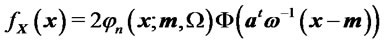 (1)
(1)
where  is the diagonal matrix
 ,
,  for
for ,
,
 is the density of a
  -random vector and
  is the cumulative distribution function of a univariate standard normal. In this case we write
 . In particular, in the univariate case,
  has the skew-normal distribution of parameters
  and
and  if for all
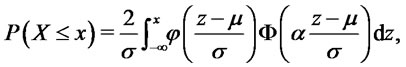
where . In this case we write
 . Clearly for
  we have
 . For
. For  the distribution is skewed and indeed its mean, variance and skewness can be easily computed. They are respectively given by:

with .
.
We refer the reader to Arellano and Azzalini ([19]) and Genton ([20]) for further properties and many interesting applications.
Let us now consider a market with  basic risky assets whose future returns, at time
 , are described by a random vector
  such that:
 (2)
(2)
An investor, the decision maker, is facing with the problem of allocating her initial capital on the market by choosing a portfolio , with
  and holding it unchanged up to time
 . The portfolio return is given by the random variable
  with:
with:
 (3)
(3)
and parameters ,
,  , and
, and
 (4)
(4)
where  and
and , see Azzalini ([18]). Henceforth it is clear that in order to compare the returns of two different portfolios
  and
and  on this market we must have at our disposal criteria which allow us to compare two univariate skew-normal random variables. In Section 4 we prove simple criteria based on stochastic dominance, Levy ([1]). Although we only make use of standard techniques, to our best knowledge these results have never been discussed in the classical literature on the subject. An investor can use them to discard a portfolio or a family of portfolios whose returns are stochastically dominated by the return of another portfolio.
3. Portfolios Including Derivative Securities in Normal Markets
In this section we briefly show how the skew-normal return distributions can naturally appear even in markets with normal returns in the primary risky assets, if in the same markets are traded derivative securities which incorporate non-linear pay-offs. More specifically consider markets for which the shape parameters of the basic risky assets are all zero ( ), that is
 (5)
(5)
and suppose that a straddle on one of the assets is available at a cost  and strike price
 . To simplify the exposition we fix
  and denote by
  and
and  the market basic risky securities; therefore their returns over the interval
  will follow the law:
 (6)
(6)
with  and
and . Let
. Let  be their present spot prices, a straddle is written on the first asset and will pay to the holder
 ,
,  denoting the asset price at maturity date
 . Consider an investor who wishes to allocate percentages of her capital both on the straddle and on shares of asset
 , while investing the remaining part on a risk-free bond. It turns out that for a strike value
  equal to
  the portfolios returns will display skew-normality. This condition on
  appears to be very stringent, however in practice we could have
  with returns distribution close to skew-normality. Notice that the case
  corresponds to a straddle traded “at the money” (this particular case, and with
 , has been discussed by Blasi ([21])). Indeed denoting by
  the percentage of initial capital invested on the straddle on asset
 , by
, by  the percentage of initial capital invested on asset
 , the return of the portfolio
 , at time
  will be
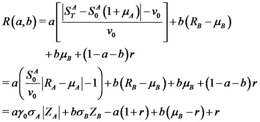 (7)
(7)
where ,
,  ,
,  is the bond yield and standardized assets returns have been denoted by
 . We notice that a decomposition analogous to (7) continues to hold also for the multi-asset case (
 ), that is for portfolios investing on a straddle on one of the assets, on shares of the remaining
  risky assets and on the risky-free asset. The following result is a straightforward generalization of a result by Henze ([22]) and can be proven by elementary methods:
Proposition 3.1 Let  be correlated
  random variables. Let
  denote the correlation coefficient,
  , and
, and  and
and  real numbers. Then the random variable
is a mixture of two skew-normally distributed random variables. Specifically, denoting by  the probability density of
 , it holds:
where
with  and
and .
.
In particular for  we have:
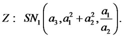
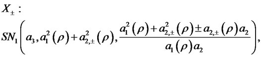
For example it is readily seen that for  the above result implies:
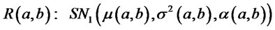 (8)
(8)
with parameters:
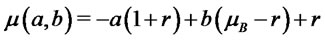 (9)
(9)
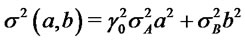 (10)
(10)
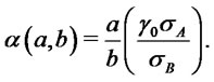 (11)
(11)
We remark that given  and the assets volatilities
  the shape parameter depends only on the ratio of the chosen allocation percentages and vanishes for
 . Shorting the straddle or the second asset produces portfolios with negative shape parameter in the returns distribution and hence with negative skewness. On the other hand positive skewness increases unboundedly as the percentage
  approaches zero. Furthermore, for the above portfolios returns distributions scale and shape parameters satisfy the relation
  , which implies that scale changes with shape. In the case
  the returns
  will be described, accordingly to the previous proposition, by a mixture of two skew-normal distributions
 , the identification of
  and
and  being straightforward. We remark that while on one hand finite mixture of normaldistributions have been already considered in the financial literature as possible flexible tool for modelling assets returns in portfolio selection problems (Buckley et al. ([23])), on the other hand finite mixture of skewnormal distributions up to now have received attention mainly in applied statistical settings, see for instance Lee et al. ([24]), but not in connection with financial applications.
An immediate consequence of the example discussed above is the fact that even in a normal market an investor can face the problem of comparing portfolios having returns which are skew-normally distributed. Once again the decision maker needs criteria which can help her allocation choice process by discarding portfolios which have dominated returns. In the next section we shall provide some simple, yet rigorous, stochastic dominance criteria.
4. Stochastic Dominance Results
We start recalling some basic definitions: given two realvalued random variables  and
and  we say that
  stochastically dominates at first order
  (FSD), and we shortly write
  if
if
 (12)
(12)
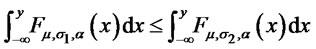
for all ; we say that
  stochastically dominates at second order
  (SSD), and we shortly write
  if
if
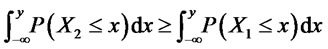 (13)
(13)
for all . More generally, a random variable
  stochastically dominates another random variable
  at the order n-th if
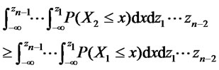
for all values . If the previous inequalities hold strictly we say that we have strict dominance. Obviously (n − 1)-th order dominance implies n-th order dominance.
The classical stochastic ordering results for univariate normal random variables  and
and  are the following (ref. Levy (2005)):
1) If  and
and  then
then ;
;
2) If  and
and  then
then 
In particular we have strict dominance for  and
and  (or
(or  and
and ).
).
To provide a generalization of these results to the skewnormal case we need the following:
Theorem 4.1:
1) Let  and
and
 . Suppose
 , then
 .
.
2) Let  and
and  . Suppose
  then
then
 .
.
3) Let  and
and . Suppose
  and
and , then
 .
.
4) Let  and
and 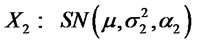 . Suppose
  and
and
 , then
 .
.
Proof.
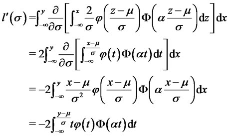
1) Let  and denote by
  the corresponding distribution function. For each fixed
  and
and  and arbitrary
  we consider the function
 . We have:
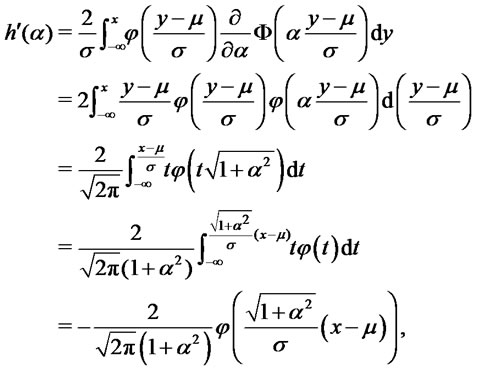
where we have used 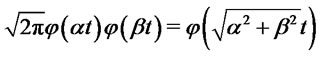
and . Therefore
  is decreasing and
  for all
 .
.
2) For each fixed  and
and  and arbitrary
  we consider the function
 . We have:
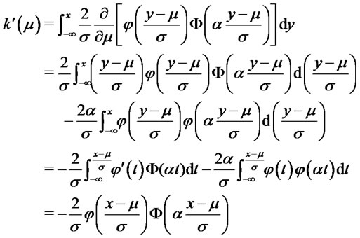
by integrating by parts the first of the two integrals.
Therefore  is decreasing and
  for all
 .
.
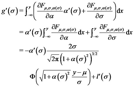
3) For each fixed  and
and  and arbitrary
  we consider the function
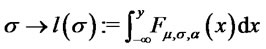 . We have:
and by integrating by parts the last integral

which is non negative for all .
.
Henceforth  is increasing,
 for all
 , and we get the result.
4) Set  then
then  and the second assumption on the parameters is equivalent to
 for
for . For each fixed
  and
and 
and arbitrary  we consider the function
  , where
 . We have:
Now , hence:
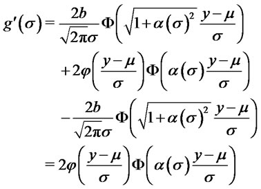
which is non negative. Henceforth  is increasing for all
 .
.
Remark: The argument by which the result (3) has been obtained fails for . In such a case
  is given by the difference of two positive quantities. The difference is positive for
  since
since . On the contrary for values of
  much larger than
  the difference is negative since the first quantity becomes much smaller than the second one. Therefore for positive
  the sign of
  is going to depend on the values of the variable
 .
.
Corollary 4.2:
1) Let  and
and
 . Suppose
  and
and then
then .
.
2) Let  and
and
 . Suppose
 ,
,  and
and
 , then
 .
.
3) Let  and
and
 . Suppose
 ,
,  and
and
 , then
 .
.
Proof.
1) Let , then by lemma 2.1 (i) and (2) we have:
2) Let  and
and then by lemma 2.1 (1), (2) and (3) we have:
3) Let , then by lemma 2.1 (2)
and (4) we have: 
Remark: a) The condition appearing in Corollary 4.2 (3) can be better understood by noticing that is equivalent to . Therefore the result can be restated in the following form: If
 ,
,  and
and  then
then .
.
b) Let 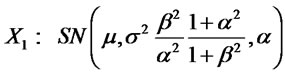 and
and
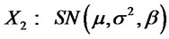 with
with . Being
  we have
  and from Corollary 4.2 (3) it follows
 . Notice that
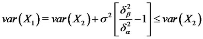 .
.
Henceforth, a larger positive skewness parameter in a financial position gives rise to an improvement over a previous position, from a stochastic dominance viewpoint, if it is accompanied by a variance reduction which leaves unchanged the skewness of the position.
c) It is well known that  if and only if
  for all non decreasing and concave functions
 . Therefore, by choosing
 , conditions (2) of Corollary 4.2 imply
 .
.
d) Consider the two-dimensional risky market discussed in Section 2 and the parametrized family of portfolios which invest on the straddle on asset , on shares of asset
 , putting all the remaining wealth on a riskfree bond. Assume
  and
and . Consider two portfolios
  and
and  and the corresponding returns
  and
and . Suppose 1)
 , 2)
, 2)
 , and 3)
 , then from (2) we get
 .
.
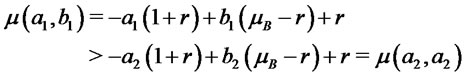
In addition from (3) we obtain . Finally from (1) we have
  and therefore
  Then by Corollary 4.2 (2) we get
 .
.
5. Acknowledgements
The authors thank the anonymous referee for useful suggestions which led to improvements in the presentation of the results. The second named author thanks Prof. A. Ramponi for advices and Centro V. Volterra for financial support.
REFERENCES
- H. Levy, “Stochastic Dominance,” Springer-Verlag, New York, 2005.
- M. W. Brandt, “Portfolio Choice Problems,” In Y. AitSahalia and L. P. Hansen, Eds., Handbook of Financial Econometrics, forthcoming.
- W. Sharpe, G. J. Alexander and G. W. Bailey, “Investments,” Prentice-Hall, Upper Saddle River, 1998.
- H. Markowitz, “Portfolio Selection,” Journal of Finance, Vol. 7, No. 1, 1952, pp. 77-91. doi:10.2307/2975974
- G. M. de Athayde and R. G. Flores, Jr., “Finding a Maximum Skewness Portfolio: A General Solution to Three Moments Portfolio Choice,” Journal of Economical Dynamics and Control, Vol. 28, No. 7, 2004, pp. 1335-1352. doi:10.1016/S0165-1889(02)00084-2
- L. Pastor, “Portfolio Selection and Asset Pricing Models,” Journal of Finance, Vol. 55, No. 1, 2000, pp. 179- 223. doi:10.1111/0022-1082.00204
- N. G. Polson, “Bayesian Portfolio Selection: An Empirical Analysis of the S & P 500 Index 1970-1996,” Journal of Business Economical Statistics, Vol. 18, No. 2, 2000, pp. 164-173. doi:10.2307/1392554
- H. Konno and H. Yamazaki, “Mean-Absolute Deviation Portfolio Optimization Model and Its Applications to Tokyo Stock Market,” Management Science, Vol. 37, No. 5, 1991, pp. 519-531. doi:10.1287/mnsc.37.5.519
- H. Markowitz, P. Todd, G. Xu and Y. Yamane, “Computation of Semivariance Efficient Sets by the Critical Line Algorithm,” Annals of Operations Research, Vol. 45, No. 1, 1993, pp. 307-317. doi:10.1007/BF02282055
- F. J. Feiring, W. Wong, M. Poon and Y. C. Chan, “Portfolio Selection in Downside Risk Optimization Approach: Application to the Hong-Kong Stock Market,” International Journal of Systems Science, Vol. 25, No. 1-3, 1994, pp. 1921-1929. doi:10.1080/00207729408949322
- F. Black and R. Litterman, “Asset Allocation: Combining Investor Views with Market Equilibrium,” The Journal of Fixed Income, Vol. 1, No. 2, 1991, pp. 7-18. doi:10.3905/jfi.1991.408013
- A. Meucci, “The Black-Litterman Approach: Original Model and Extensions,” The Encyclopedia of Quantitative Finance, Wiley, New York, 2010.
- C. J. Adcock and K. Shutes, “Portfolio Selection Based on the Multivariate Skewed Normal Distribution,” In: A. Skulimowski, Ed., Financial Modelling, Progress & Business Publishers, Krakow, 2001
- C. Harvey, J. Liechty, M. Liechty and P. Muller, “Portfolio Selection with Higher Moments,” Quantitative Finance, Vol. 10, No. 5, 2010, pp. 469-485. doi:10.1080/14697681003756877
- C. J. Adcock, “Exploiting Skewness to Built an Optimal Hedge Fund with a Currency Overlay,” European Journal of Finance, Vol. 11, No. 5, 2005, pp. 445-462. doi:10.1080/13518470500039527
- J. F. Bacmann and S. Massi-Benedetti, “Optimal Bayesian Portfolios of Hedge Funds,” International Journal of Risk Assessment and Management, Vol. 11, No. 12, 2009, pp. 39-57. doi:10.1504/IJRAM.2009.022196
- T. Post, “Empirical Tests for Stochastic Dominance Efficiency,” Journal of Finance, Vol. 58, No. 5, 2003, pp. 1905-1931. doi:10.1111/1540-6261.00592
- A. Azzalini, “The Multivariate Skew-Normal Distribution and Related Multi-Variate Families (with Discussion),” Scandinavian Journal of Statistics, Vol. 32, 2005, pp. 159- 188. doi:10.1111/j.1467-9469.2005.00426.x
- R. B. Arellano and A. Azzalini, “The Centered Parametrization for the Multivariate Skew-Normal Distribution,” Journal of Multivalent Analysis, Vol. 99, 2008, pp. 1362- 1382. doi:10.1016/j.jmva.2008.01.020
- M. G. Genton, “Skew-Elliptical Distributions and Their Applications: A Journey beyond Normality,” Chapman & Hall/CRC, Boca Raton, 2004. doi:10.1201/9780203492000
- F. S. Blasi, “Black-Litterman Model in a Skew-Normal Market,” Statistical Computation and Complex Systems 2009, Milan, 14-16 September 2009.
- N. Henze, “A Probabilistic Representation of the ‘SkewNormal’ Distribution,” Scandinavion Journal of Statistics, Vol. 13, 1986, pp. 271-275.
- I. Buckley, D. Saunders and L. Seco, “Portfolio Optimization When Asset Returns Have the Gaussian Mixture Distribution,” European Journal of Operational Research, Vol. 185, No. 3, 2008, pp. 1434-1461. doi:10.1016/j.ejor.2005.03.080
- T. I. Lin, J. C. Lee and S. Y. Yen, “Finite Mixture Modelling Using the Skew-Normal Distribution,” Statistica Sinica, Vol. 17, No. 3, 2007, pp. 909-927.
NOTES
*GDF-SUEZ Trading [The present paper expresses only the authors own views and in absolute no way represents opinions of GDF-SUEZ Trading or its Management Board].