Applied Mathematics
Vol. 4 No. 10 (2013) , Article ID: 37850 , 14 pages DOI:10.4236/am.2013.410193
Explicit Approximation Solutions and Proof of Convergence of the Space-Time Fractional Advection Dispersion Equations
Department of Mathematics and Computer Science, Faculty of Science, Suez Canal University, Ismailia, Egypt
Email: entsarabdalla@hotmail.com
Copyright © 2013 E. A. Abdel-Rehim. This is an open access article distributed under the Creative Commons Attribution License, which permits unrestricted use, distribution, and reproduction in any medium, provided the original work is properly cited.
Received June 29, 2013; revised July 29, 2013; accepted August 6, 2013
Keywords: Advection-Dispersion Processes; Grünwald-Letnikov Scheme; Explicit Difference Schemes; Caputo Time-Fractional Derivative; Inverse Riesz Potential; Random Walk with and without a Memory; Convergence in Distributions; Fourier-Laplace Domain
ABSTRACT
The space-time fractional advection dispersion equations are linear partial pseudo-differential equations with spatial fractional derivatives in time and in space and are used to model transport at the earth surface. The time fractional order is denoted by  and
and  is devoted to the space fractional order. The time fractional advection dispersion equations describe particle motion with memory in time. Space-fractional advection dispersion equations arise when velocity variations are heavy-tailed and describe particle motion that accounts for variation in the flow field over entire system. In this paper, I focus on finding the precise explicit discrete approximate solutions to these models for some values of
  with
with ,
,  while the Cauchy case as
  and the classical case as
  with
with  are studied separately. I compare the numerical results of these models for different values of
 ![]() and
and  and for some other related changes. The approximate solutions of these models are also discussed as a random walk with or without a memory depending on the value of
 . Then I prove that the discrete solution in the Fourierlaplace space of theses models converges in distribution to the Fourier-Laplace transform of the corresponding fractional differential equations for all the fractional values of
 ![]() and
and .
.
1. Introduction
The development which has happened on the last twentyfive years on the fractional calculus opened many new applications on many fields such as physics, hydrodynamics, chemistry, financial mathematics, and some other fields. Actually a growing number of articles and books which are interesting on this field and its applications have appeared in these last 25 years (see for example: [1-5] and see also my thesis [6]. Fractional in time means that the first-order time derivative is replaced by the Caputo derivative of order , see [4]. Fractional in space means replacing the second order space-derivative is replaced by the Feller operator [7] in the symmetric case with order
 .
.
The behaviour of particles in transport under the earth surface is an important problem. For examples, the transport of solute and contaminant particles in surface and subsurface water flows, the behaviour of soil particles and associated soil particles, and the transport of sediment particles and sediment-borne substances in turbulent flow. There are many other examples in this field. The classical advection dispersion equation, ade, has been used to formulate such problems. The generalized fractional advection-dispersion equation, fade, has recently gotten an increasing interest from many scientists because it has many applications specially on studying the transport of passive tracers carried by fluid flow in a porous medium, see Benson, Meerschaert et al. [8-12]. In their work they gave applications and experimental results for the space-fade.
There is no unique solution for the space-time fractional diffusion processes but there are some attempts using different forms of the hyper geometric functions, as for example: in [13] the authors attempted to find an analytical solution for other special form of the fractional, see also [14,15]. Therefore authors who study modelling of fractional processes use some developed methods to descritize the fractional operators. For examples, in [16], the authors used their own method of descretization to find the approximate solution of the space-fade and gave some numerical results. In [17], the authors studied the approximate solution of the space-fade, for  and
and , only using the backward Grünwald-Letnikov Scheme. The backward Grünwald-Letnikov Scheme has been successfully adopting by Gorenflo, Mainrdi, and etal, see [4,18,19] for modelling space-fractional diffusion processes. Also has been used by Gorenflo and E. A. Abdel-Rehim, see [20-24] for modelling time-fractional Fokker-Planck equations and their convergence in the Fourier Laplace domain.
I am interested in this paper to find the approximate solutions of the space-time fractional advection equation, space-time fade, by adopting the backward GrünwaldLetnikov Scheme joined with the common finite difference methods. The space-time fade is considered as a diffusion process under the action of a constant force in a fractal medium with a memory. I study and numerically investigate the effect of the time fractional on the path of the particle motion as well as the effect of the spacefractional order for the three cases as: 0 < α < 1, 1 < α < 2, and . I compare between all these cases numerically. My numerical results are consistent with the results of [17] for the studied case
  and
and . The approximate solutions according to the values 1 < α < 2, and
  joined with
  are firstly studied on this paper. The proof of the convergence in distribution for each case is also considered. Therefore this paper is organized as follows: Section 1 is denoted to the introduction; Section 2 is devoted to the definitions of the used fractional operators and their Laplace-Fourier transformations; and Section 3 introduces the classical case
 . Section 4, the fractional in time α = 2,
  , is studied. Section 5.1 is denoted to the case
 , and
, and  is studied at Section 5.2. Section 6 is devoted to the caseα = 1,
 . Finally, the numerical results will be displayed and explained in Section 7 and one compares these results with the results of the given references.
2. Important Definitions and the Outline of the Proof of Convergence in Distribution
The generalized fade reads
 (2.1)
(2.1)
Here a, and b are positive constants representing the dispersion coefficient, and the average fluid velocity and it acts as the drift term to the right respectively. My aim is to give the approximation solutions of the space-time fad equations for all values of ![]() and
and . I study also the convergence of the approximation solutions to the solutions of the corresponding analytical solutions of the space-time fad equations in the Fourier-Laplace domain.
The used time-fractional derivative operator 
is called Caputo fractional operator, see [4] to know the relation between Caputo fractional derivative and the famous Riemann-Liouville fractional derivative operators. Caputo fractional derivative in the Laplace domain reads

This equation is important for solving the fractional differential equations because it show the dependence on the initial conditions. Here  is called the Riesz space-fractional differentiation operator. I adopt here the notation introduced by [25]. It is formally a power of the positive definitive operator
 and must not be confused with a power of the first order differential operator
  (see [4] for a detailed theory of this operator and related operators). I need to adopt the Fourier transform of a (generalized) function
 ,
,  , which is defined as
For the proof of convergence in distribution I need to use the Fourier transform of  which reads
 (2.2)
(2.2)
while
 (2.3)
(2.3)
This means, in the Zaslavski’ s notations,
 (2.4)
(2.4)
From (2.2) - (2.4), one easily sees that in the case 

Since , we can set
 which proves that the Riesz derivative is a symmetric fractional generalization of the second derivative. For more information about the Fourier transform and the pseudo-differential operators as semi groups of linear operators, see e.g. [26,27]. In my paper, I discuss the approximate solution of the Equation (2.1) for all values of
 ![]() and
and , to do so, I descretize
 ![]() and
and  by the grid
  with
with ,
,
 . Here
 , and
, and  are the steps in space and in time, respectively, and
  is the number of steps at the x direction. Treating
  as a density of an extensive quantity (like mass, charge, solute concentration, or probability), the approximation of the collected quantity
  presents in a spatial cell
  at the instant
  by a clump
 ,
,
 (2.5)
(2.5)
For , I introduce the column vector

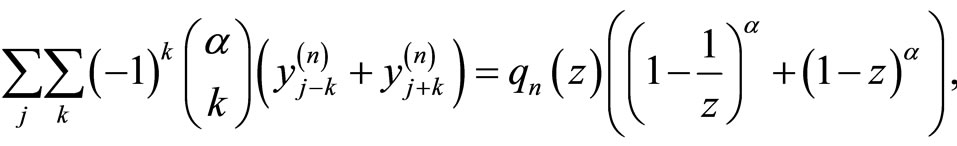
where . To proceed on the proof of convergence in distribution, one needs to use the method of generating functions, see [22] for more information about the procedures used to prove the convergence. Therefore, for
 , define
 (2.6)
(2.6)
for the sequence of clumps
 . Using the initial conditions, I introduce the function
and applying the Fourier-transform, we obtain
 (2.7)
(2.7)
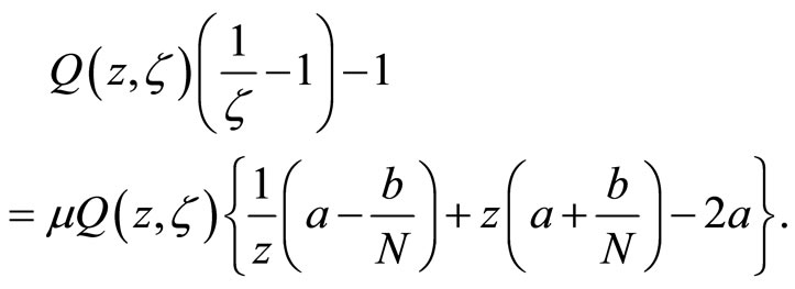
Now, introduce the bivariate (two-fold) generating function
 (2.8)
(2.8)
as a function of![]() , where
, where , for the sequence
 (2.9)
(2.9)
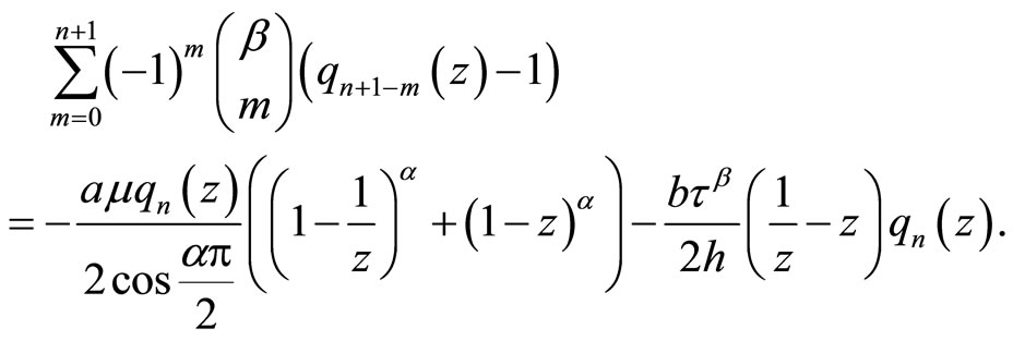
Introduce the function  and apply the Laplace-transform, one gets
 (2.10)
From Equations (2.7) and (2.10), we deduce that if we replace  by
by  and
and ![]() by
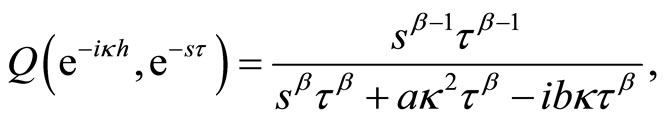
by , in Equation (2.8), we get the Fourier-Laplace transform of the bivariate sequence
  which is obtained by collecting all the sequences in (2.9). This means
 (2.11)
Our aim now is to prove that  is related asymptotically to the Fourier-Laplace transform of
  which represents the analytical solution of Equation (2.1) for any values of
 ![]() and
and , and for a fixed
  and
and , as
, as![]() . So far, I will prove
. So far, I will prove
 (2.12)
for each case.
3. The Classical ade
I describe in this section the classical partial differential ade and its proof of convergence in distribution. It is well known that the classical ade is a partial differential equation describing the solute transport in aquifers and it reads
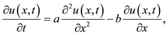 (3.1)
(3.1)
here  is the solute concentration. The conditions imposed on the solution
  are
are

With the initial condition . The classical ade is also interpreted as a deterministic equation with the probability function
  which describes the particle spreading away from the plume center of mass. The stochastic process
  described by Equation (3.1) is a Brownian motion with a constant drift [11].
If , then one has the diffusion of a free particle, that is, a particle in which no forces other than those due to the molecules of the surrounding medium are actingwhich reads
 . It has the solution
 . Consequently by using the Galilei transformation of the independent variables
  to
to , then the solution of (3.1), as
 is
is . In the Fourier domain
 and hence fourth in the FourierLaplace domain, see [28]
 (3.2)
(3.2)
Now descretizing (3.1) by the central symmetric difference in space and forward in time, one gets
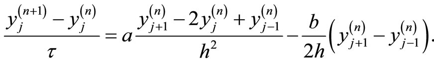 (3.3)
(3.3)
Introduce the scaling relation
 (3.4)
(3.4)
and for the positivity of all the coefficients of , one must put
 . Now let
 , one can write
  as
as
 (3.5)
(3.5)
The discrete solution at Equation (3.5) describes also a random walk with sojourn probability  of a particle at the point
  at the instant
 ![]() and it may jump either to the points
and it may jump either to the points ,
,  , or
, or  at the time instant
 , see [29]. Utilizing this concept, Equation (3.5) can be rewritten as
 (3.6)
(3.6)
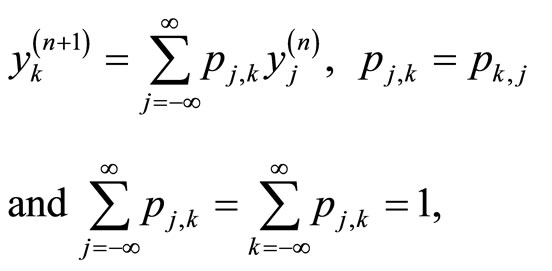
The transition probabilities ,
,  and
and  in Equation (3.6) satisfy the essential condition

Now one can use these transition probabilities to constitute a tridiagonal, P matrix, in which
 . Therefore, Equation (3.5) is written in the following matrix form
 (3.7)
(3.7)
Introduce the row vector , defined as

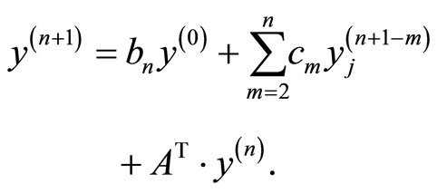
In order to find the explicit discrete solution of Equation (3.1), I have to take the transpose of each sides of the matrix Equation (3.7) and rewrite it as
 (3.8)
(3.8)
and for the numerical calculations, it is convenient to write the stochastic matrix  in the form
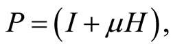 (3.9)
(3.9)
here I is the unit matrix and  is a
is a  matrix whose rows are summed to zero. In Section 7, I give the evolution of
  for different values of
 . Now I am going to prove that the discrete solution at Equation (3.5) converges to the Fourier-Laplace transform of Equation (3.1). Rewrite Equation (3.5) as
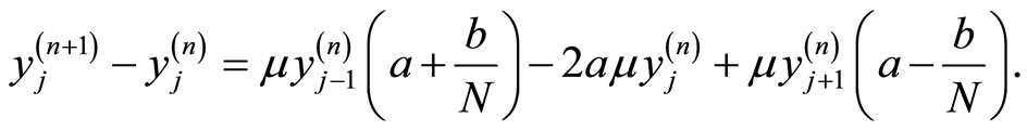 (3.10)
Then multiplying both sides by  and summing over all
 , to get
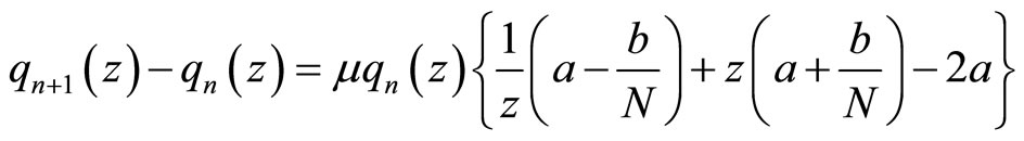 (3.11)
Multiplying both sides by  and summing over all
 , one gets
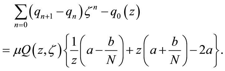
The choice of the initial condition of the column vector  satisfying that
 , guarantees that
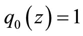
 (3.12)
Now, replace  by
by  and
and ![]() by
by , in Equation (3.12), to get

Now after using Taylor expansion and taking the limits as  and
and , one gets

Compare this equation with Equation (3.2), then Equation (2.12), is satisfied for the classical ade.
4. The Time-Fractional ade
In this section, I replace the first-order time derivative in Equation (3.1) by the Caputo fractional derivative,
 , with
 . Then this generalized time-fractional advection-dispersion equation, fade, reads
 (4.1)
(4.1)
For more information about the Caputo fractional derivative and its relations to the Riemann-Liouville, see [6] and the list of references therein. Now, Taking the Fourier-Laplace transform, see Section 2, one gets
 (4.2)
(4.2)
To descretize , I utilize the backward Grünwald-Letnikov scheme which has been successfully utilizing at [19-24] for modelling and simulating the timefractional diffusion processes and the time-fractional Fokker-Planck equations.
 (4.3)
(4.3)
Join this discretization with the common symmetric finite difference for  and
and , then one has
 (4.4)
(4.4)
Now introduce the scaling parameter
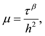 (4.5)
(4.5)
and solve for , one gets
 (4.6)
(4.6)
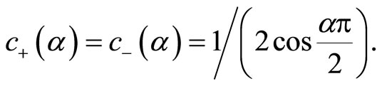
where for ease of writing, I use  and
and  which has been originally introduced in [19] as
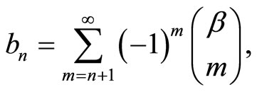
with , and all
 ,
, . Finally,
  and
and  satisfy the relation
 (4.7)
(4.7)
where , see [19]. For all the coefficients of
to be positive, it is required that . Rewrite Equation (4.6) in the following form
 (4.8)
(4.8)
This equation can be interpreted as a random walk with a memory, see [30]. In this case, the particle is sitting at the position  at the time instant
 ![]() and can move to either
and can move to either ,
,  , or
, or  at the time instant
 . It has also the possibility to return back to
  at any of the time instants
 . By using the identity (4.7), it is easily to prove that the summation of the transition probabilities at the right hand side of Equation (4.8) equals to one. These transitions constitute a symmetric random walk. Now, constitute the column vector
 , then Equation (4.6) is written in the matrix form
 (4.9)
(4.9)
where  is
is  matrix and is not a stochastic matrix as its rows are summed to
 , where
 . A useful numerical method to ease the computation is to write the matrix
  as
as

where  is the same matrix defined in the last section, i.e. it does not depend on the value of
  then it does not depend on the time. In Section
 , I compare the evolution of
  for different values of
  and
and .
.
Now, I want to prove that the discrete solution (4.6), in the Fourier-Laplace domain as  and
and , converges to the Fourier-Laplace transform of Equation (4.1). To do so, I have to adopt the initial condition which satisfies that
 , then
 . Then multiply each sides of Equation (4.4) by
  and sum over all
 , to get
 (4.10)
Now proceed further, multiply each sides by  and sum over all
![]() , to get
, to get
 (4.11)
For manipulating the R.H.S., one needs to use the rule of multiplication of two sequences  and
and , see Feller [29], in which

After using this rule, and put , then apply Taylor expansion, and take the limit as
 , one gets

Now, substitute , then again apply Taylor expansion, and take the limit as
 , you get
then multiply each sides by![]() , one gets
, one gets

Then I have proved the required aim for the timefractional ade.
5. The Space-Time-Fractional ade
In this section I consider the space-time fade, Equation (2.1). It is known that the space-fractional ade arises when velocity variations are heavy tailed and describe particle motion that accounts for variation in the flow field over entire system. The time fractional ade arises as a result of power law particle residence time distributions and describe particle motion with memory in time, see
[12]. The used space-fractional operator , is the symmetric Feller operator, see [7]. This operator represents the negative inverse of the Riesz Potential
  whose symbol is
 , i.e.

where the symmetric Riesz Potential operator is defined as

where
 (5.1)
(5.1)
The Fourier-Laplace transformation of Equation (2.1) reads
 (5.2)
(5.2)
When descretizing the Riesz fractional operator 
one must use a suitable finite difference scheme and exclude the case . To do so, I use the approximation of the inverse operators
  by the Grünwald-Letnikov scheme, see Oldham & Spanier [31], Ross & Miller [1] and see also [6], in which one can find a long list of related references. The inverse of the Riemann-Liouville integrals can formally be obtained as the limit
 (5.3)
(5.3)
where  denotes the approximating Grünwald-Letnikov scheme which reads, see [4,18,19]
a) 
 (5.4)
(5.4)
b) 
 (5.5)
(5.5)
The shift in the index  in Equation (5.5) is required to obtain a scheme with all coefficients are non-negative in the final formula for
  which gives schemes for simulating particle paths which results after replacing the second order space-derivative in Equation (4.1) by the Feller operator [7]. One can adopt, for simplicity, the notation introduced by Zaslavski [25].
 (5.6)
(5.6)
one must distinguish the descretization of ![]() with respect to the value of
with respect to the value of![]() , as follows:
, as follows:
 (5.7)
(5.7)
while
 (5.8)
(5.8)
Now we adjoin the descretization of , with the descretization of
 , and with the finite sequence
 . In what follows, I give the descretization of the space-time fractional ade for each case.
5.1. Case (a): ,
, 
In order to ensure that all the coefficients of I have to descritize
  by using the symmetric central scheme, so the discretization of Equation (2.1) reads
 (5.9)
(5.9)
Adopting the scaling relation
 (5.10)
and using Equation (5.1), one can solve Equation (5.9) for  to get
 (5.11)
To ensure that the coefficients of all , it requires that

Let us write Equation (5.11) in the form of a random walk, in which the walker is sitting at  at
at ![]() and jumps to
and jumps to  at
at , where
see [32] for more information about the discrete random walk of space-fractional diffusion processes. Then by using this notations, Equation (5.11) can be written in the form of random walk as
 (5.12)
The first two terms at the LHS of this equation represent the memory part and the other terms represent the diffusion under the drift term. I like to write  as it represents the transition to the next step at the same point,
  represents jumping one step to the left,
  represents jumping one step to the right, and similarly
  jumping
  steps to the left or right. By using the identity (4.7), and the identity

then it is easily to prove that the summation of all the transition probabilities is one.
Now for the numerical calculations, and since there is a symmetric random walk, I adjust  and ignore all the transitions outside this interval. So it is convenient to write the last equation in the form of a matrix form
 (5.13)
Here  is an elegant
  fifth diagonal matrix with its elements are computed as
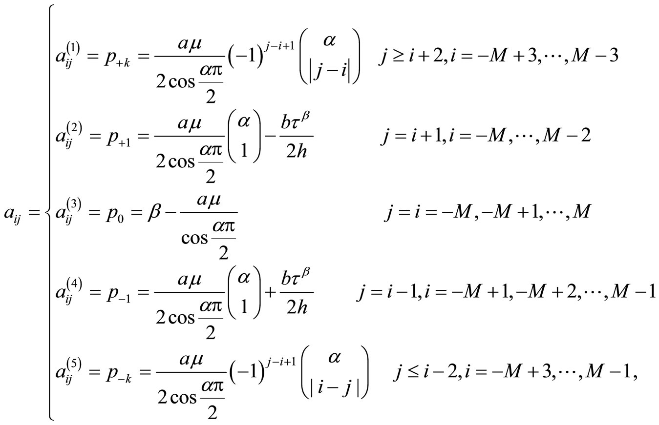 (5.14)
where  and
and . In the special case as
 , one recovers the well-known three point jumps of the classical ade because
  as
as , and hence the matrix
  be the same as matrix
 ![]() defined in Equation (3.7). In Section 7, I will plot the path of the particle representing by (5.13). Now, I will prove that the discrete solution at (5.9) converges in the Fourier-Laplace domain to the Fourier-Laplace transform of Equation (2.1) as
defined in Equation (3.7). In Section 7, I will plot the path of the particle representing by (5.13). Now, I will prove that the discrete solution at (5.9) converges in the Fourier-Laplace domain to the Fourier-Laplace transform of Equation (2.1) as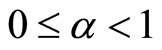 . To do so, multiplying both sides of Equation (5.9) by
  where and sum over all
 , where it is easy to prove
then one gets
 (5.15)
The second step is to multiply both sides of this equation by  and sum over all
![]() ,
,

then put  and
and  and use the previous results. The only new part on the proof is as
 , one can easily prove by using the fundamentals of complex analysis that

So far

Finally multiply each side by ![]() and substitute the value of
and substitute the value of , and compare with (5.2), one gets

So, I proved the desired aim.
5.2. Case (b): ,
, 
I have to descritize  by using the backward difference scheme, in order to ensure that all the coefficients of
  are positive for
 . Then the descretization of the space-time fade in this case reads
 (5.16)
After using the scaling relation (5.10), I am going to separate the coefficients related to  from the last summation and rearrange Equation (5.16) as
 (5.17)
To ensure that all the coefficients of  are positive, the scaling relation must satisfy
It is known as , the value of
 and that ensure that
 . I can use the same symbols of the last subsection to write this equation in the form of the random walk as
 (5.18)
Again the summation of all the transition probabilities of this equation over all  is one. As in the previous, Equation (5.17) can be written in the same matrix form (5.13) where the diagonal elements of the matrix
  are defined as (see (5.19) below)
 (5.19)
 In the numerical calculations, I plot the path of the particle for different values of . I choose the values of
  according to condition of each case. The situation as
  is the same as the previous cases. Now, I am going to prove the convergence of the discrete solution (5.18) in the Fourier-Laplace domain to the solution of the space-time fade as
 . To do so, one has to shift the indices of
  and rewrite Equation (5.18) as
 (5.20)
Again multiply each side by  and sum over all j and use all the identities of the last section, to get
 (5.21)
Replace , where, it is clear that

So one gets

Now, multiply both sides by ,
,  , and sum over all
![]() , to get
, to get

Finally, replace ![]() by
by , solve for
 , and multiply both sides by
![]() , you will get the desired aim
, you will get the desired aim , Equation (5.2). Then the discrete solution converges to the solution of its corresponding space-time fade in the Fourier-Laplace domain.
6. The Discretization of the Space-Time Fade as ,
, 
The Cauchy fractional ade needs a special treatment. I am going to prove first the convergence of the discrete solution. Therefore, the Fourier-Laplace transformation of the space-time fade (2.1), as , reads
 (6.1)
(6.1)
This case is related to the Cauchy distribution and one cannot use the Grünwald-Letnikov discretization of 
at Equations (5.7) and (5.8) because the denominator is zero and  for
for . Instead of GrünwaldLetnikov discretization, one must use the descretization used in [33]. The authors of [33] deduced the descretization of
  from the Cauchy density
 , see
, see
[6] for more information. They replaced the factor
 ,
,  , in Equations (5.7) and (5.8) by
  for
for , and
, and  for
for . Therefore by using the scaling parameter
 (6.2)
(6.2)
one gets
 (6.3)
(6.3)
As the previous cases,  can be written in the form of a random walk with a memory as
 (6.4)
(6.4)
To have all the coefficients of  are positive, one should restrict the values
  as
as . Following
[33], it can be proved that the summations of the transition probabilities of Equation (6.4) are summed to one and one can easily write it in the form of a random walk as the previous cases. The last equation could also be written on the same matrix form (5.13). Where  is a fifth diagonal matrix whose diagonal elements are defined as
 (6.5)
(6.5)
The numerical result of this model is discussed in the next section. Noting that the coefficient ![]() and
and  play here a significant role. To prove the convergence, multiply each side of Equation (6.3) by
  and sum over all
 , then use the identity

to get
 (6.6)
(6.6)
Replace, z by , and use the identity

Finally replace, ![]() by
by  and take the limit as
 , you get
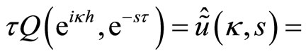 , Equation (6.1).
7. Numerical Results
In this section, I give the numerical approximate solutions for Equation (2.1). I give the evolution of  with different values of
 ![]() such, different values of the space fractional order
such, different values of the space fractional order ![]() and different values of the time fractional order
and different values of the time fractional order . I fix the values of
  while
while  and
and , with the initial condition
  as it must satisfy
 . Since
 , then the iteration index
  while
while ![]() is calculated from the scaling parameter of the specified model and its values are varying according to the restriction put on
is calculated from the scaling parameter of the specified model and its values are varying according to the restriction put on . Since I used the explicit discrete scheme, therefore, sometimes I need a huge number of steps for calculating
  specially for
 . I calculate most of the numerical results for
  and
and  but as
  and 1 < α < 2 I used
  to ensure that all the elements must be
 , because
  is probability transition matrices. To ease comparing the numerical results, I wrote the values of
![]() ,
,  and their corresponding
  with the values of
  at the figure. The classical case, i.e. as
  and
and , is plotted at Figures 1 and 2 and one can observe how rapidly the paths diffuse as the time increases. The time-fractional ade is simulated at Figures 3 and 4, i.e. for
  and
and . Figures 5, 6 are corresponding to the space-time fractional ade as 0 < α < 1 and
 . While Figures 7 and 8 are denoted for 0 < α < 1 and
 . Figures 9 and 10 are corresponding to 1 < α < 2 and
  at Figures 11 and 12 for 1 < α < 2 and
 . Finally, I plot the space-time fractional ade as
  and
and  is plotted at Figures 13 and 14. The numerical results of this paper as
  and
and  are consistent with the results at [17]. The numerical solution for the case
  and
and , i.e., the classical case in this paper is seemed perfect when comparing with the other references as it has been
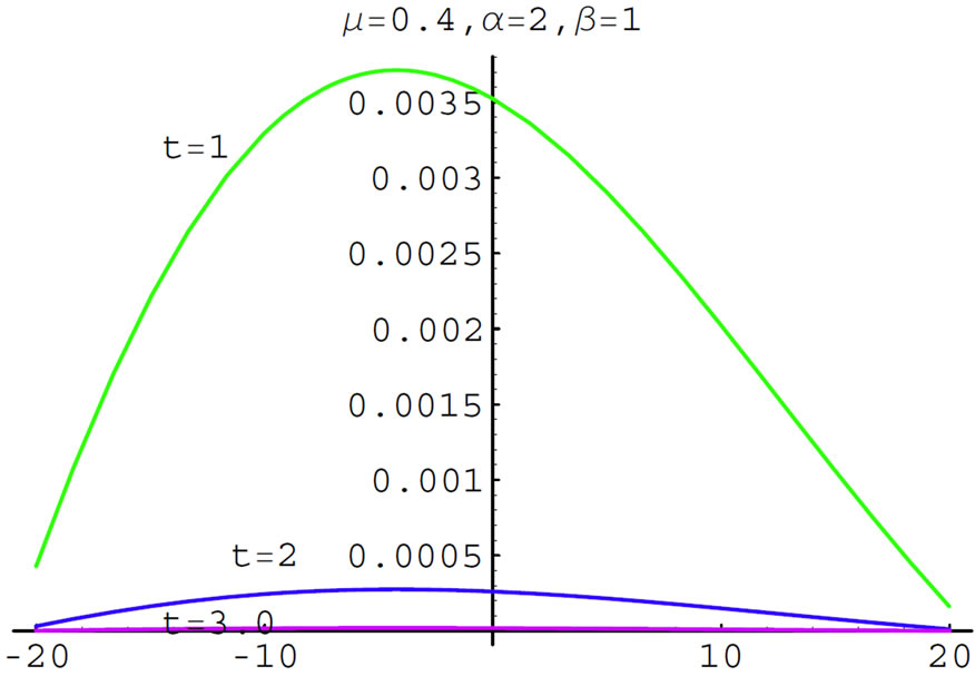
Figure 1. The classical case.

Figure 2. Classical case.

Figure 3. Time-fractional.

Figure 4. Space-time-fractional.

Figure 5. Space-fractional.

Figure 6. Space-fractional.
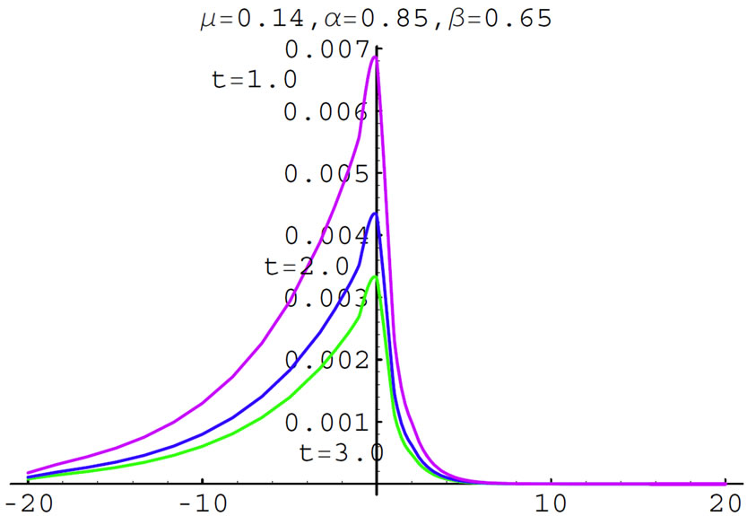
Figure 7. Space-time-fractional.

Figure 8. Space-time fractional.

Figure 9. Space-fractional.
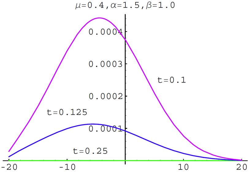
Figure 10. Space-fractional.

Figure 11. Space-time fractional.
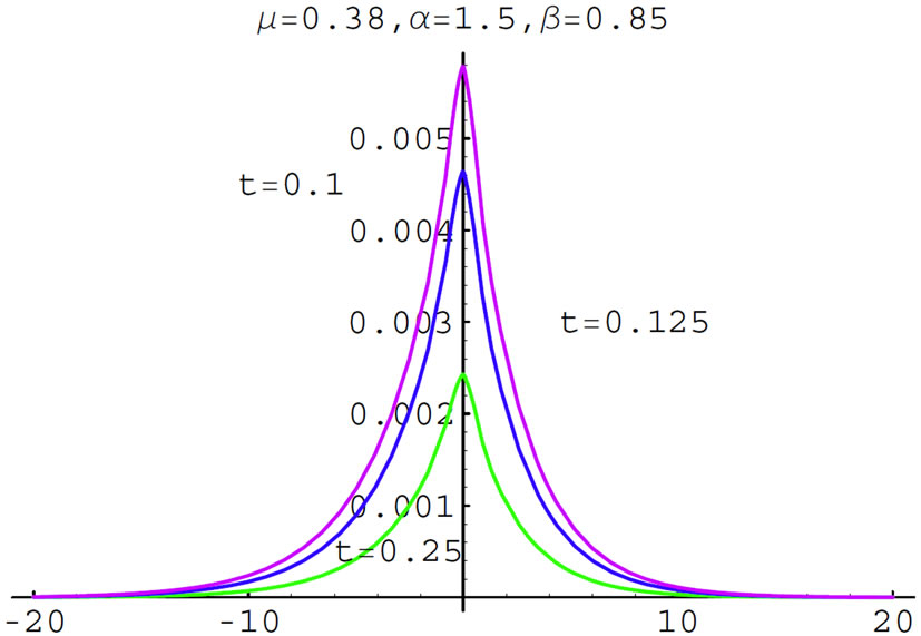
Figure 12. Space-time fractional.

Figure 13. The singular case.
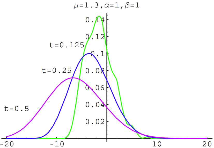
Figure 14. The singular case.
discussed by many authors. The pates as  are different than the paths corresponding to
 . The pathes for
  need a huge number of time steps to calculate them as I use the explicit difference methods.
REFERENCES
- K. S. Miller and B. Ross, “An Introduction to the Fractional Calculus and Fractional Differential Equations,” John Wily and Sons, INC., New York, Chichester, Brisbane, Toronto, Singapore, 1993.
- I. Podlubny, “Fractional Differential Equations,” Academic Press, San Diego, Boston, New York, London, Sydney, Tokyo, Toronto, 1999.
- S. G. Samko, A. A. Kilbas and O. I. Marichev, “Fractional Integrals and Derivatives (Theory and Applications),” Gordon and Breach, New York, London, and Paris, 1993.
- R. Gorenflo and F. Mainardi, “Fractional Calculus: Integral and Differential Equations of Fractional Order,” In: A. Carpinteri and F. Mainardi, Eds., Fractals and Fractional Calculus in Continuum Mechanics, Springer Verlag, Wien and New York, 1997, pp. 223-276. http://www.fracalmo.org
- N. U. Prabhu, “Stochastic Processes (Basic Theory and Its Applications),” The Macmillan Company, New York, Collier-Macmillan Limited, London, 1965.
- E. A. Abdel-Rehim, “Modelling and Simulating of Classical and Non-Classical Diffusion Processes by Random Walks,” Mensch&Buch Verlag, 2004. http://www.diss.fu-berlin.de/2004/168/index.html
- W. Feller, “On a Generalization of Marcel Riesz’ Potentials and the Semi-Groups Generated by Them,” In: Meddelanden Lunds Universitetes Matematiska Seminarium (Comm. Sém. Mathém. Université de Lund), Tome Suppl. dédié a M. Riesz, Lund, 1952, pp. 73-81.
- M. M. Meerschaert and C. Tadjeran, “Finite Difference Approximations for Fractional Advection-Dispersion Flow Equation,” Journal of Computational and Applied Mathematics, Vol. 172, No. 1, 2004, pp. 65-77. http://dx.doi.org/10.1016/j.cam.2004.01.033
- D. A.Benson, S. W. Wheatcraft and M. M. Meerschaert, “Application of a Fractional Advection-Dispersion Equation,” Water Resource Research, Vol. 36, No. 6, 2000, pp. 1403-1412. http://dx.doi.org/10.1029/2000WR900031
- D. A. Benson, R. Schumer, M. M. Meerschaert and S. W. Wheatcraft, “Fractional Dispersion, Lévy Motion, and the MADE Tracer Tests,” Transport in Porous Media, Vol. 42, No. 1-2, 2001, pp. 211-240. http://dx.doi.org/10.1023/A:1006733002131
- B. Baeumer, D. A. Benson, M. M. Meerschaert and S. W. Wheatcraft, “Subordinated Advection-Dispersion Equation for Contaminant Transport,” Water Resource Research, Vol. 37, No. 6, 2001, pp. 1543-1550.
- R. Schumer, M. M. Meerschaert and B. Baeumer, “Fractional Advection-Dispersion Equations for Modeling Transport at the Earth Surface,” Journal of Geophysical research, Vol. 114, No. F4, 2009. http://dx.doi.org/10.1029/2008JF001246
- F. Huang and F. Liu, “The Fundamental Solution of the spaace-time Fractional advection-dispersion Equation,” Journal of Applied Mathematics and Computing Vol. 18, No. 1-2, 2005, pp. 339-350.
- Y.-S. Park and J.-J. Baik, “Analytical Solution of the Advection-Diffusion Equation for a Ground-Level Finite Area Source,” Atomspheric Environment, Vol. 42, No. 40, 2008, pp. 9603-9069. http://dx.doi.org/10.1016/j.atmosenv.2008.09.019
- D. K. Jaiswal, A. Kumar and R. R. Yadav, “Analytical Solution to the One-Dimensional Advection-Diffusion Equation with Temporally Dependent Coefficients,” Journal of Water Resource and Protection, Vol. 3, No. 1, 2011, pp. 76-84. http://dx.doi.org/10.4236/jwarp.2011.31009
- Y. Xia, J. C. Wu and L. Y. Zhou, “Numerical Solutions of Time-Space Fractional Advection-Dispersion Equations,” ICCES, Vol. 9, No. 2, 2009, pp. 117-126.
- Q. Liu, F. Liu, I. Turner and V. Anh, “Approximation of the Lévy-Feller Advection-Dispersion Process by Random Walk and Finite Difference Method,” Journal of Computational Physics, Vol. 222, No. 1, 2007, pp. 57-70. http://dx.doi.org/10.1016/j.jcp.2006.06.005
- F. Mainardi, Y. Luchko and G. Pagnini, “The Fundamental Solution of the Space-Time Fractional Diffusion Equation,” Fractional Calculus and Applied Analysis, Vol. 4, No. 2, 2001, pp. 153-192. www.fracalmo.org
- R. Gorenflo, F. Mainardi, D. Moretti and P. Paradisi, “Time-Fractional Diffusion: A Discrete Random Walk Approach,” Nonlinear Dynamics, Vol. 29, No. 1-4, 2002, pp. 129-143. http://dx.doi.org/10.1023/A:1016547232119
- R. Gorenflo and E. A. Abdel-Rehim, “Discrete Models of Time-Fractional Diffusion in a Potential Well,” Fractional Calculus and Applied Analysis, Vol. 8, No. 2, 2005, pp. 173-200.
- R. Gorenflo and E. A. Abdel-Rehim, “From Power Laws to Fractional Diffusion: The Direct Way,” Vietnam Journal of Mathematics, Vol. 32, No. SI, 2004, pp. 65-75.
- R. Gorenflo and E. A. Abdel-Rehim, “Convergence of the Grünwald-Letnikov Scheme for Time-Fractional Diffusion,” Journal of Computational and Applied Mathematics, Vol. 205, No. 2, 2007, pp. 871-881. http://dx.doi.org/10.1016/j.cam.2005.12.043
- R. Gorenflo and E. A. Abdel-Rehim, “Simulation of Continuous Time Random Walk of the Space-Fractional Diffusion Equations,” Journal of Computational and Applied Mathematics, Vol. 222, No. 2, 2008, pp. 274-285. http://dx.doi.org/10.1016/j.cam.2007.10.052
- E. A. Abdel-Rehim, “From the Ehrenfest Model to TimeFractional Stochastic Processes,” Journal of Computational and Applied Mathematics, Vol. 233, No. 2, 2009, pp. 197-207. http://dx.doi.org/10.1016/j.cam.2009.07.010
- A. I. Saichev and G. M. Zaslavsky, “Fractional Kinetic Equations: Solutions and Applications,” Chaos, Vol. 7, No. 4, 1997, pp. 753-764. http://dx.doi.org/10.1063/1.166272
- J. A. Goldstein, “Semigroups of Linear Operators and Applications,” Oxford University Press, Oxford and New York, 1985.
- N. Jacob, “Pseudo-Differential Operators and Markov Processes,” Akademie Verlag, Berlin, 1996.
- R. Metzler, J. Klafter and I. M. Sokolov, “Anomalous Transported in External Fields: Continuous Time Random Walks and Fractional Diffusion Equations Extended,” Physical Review E, Vol. 48, No. 2, 1998, pp. 1621-1633. http://dx.doi.org/10.1103/PhysRevE.58.1621
- W. Feller, “An Introduction to Probability Theory and Its Applications,” Vol. 2, Johon Wiley and Sons, New York, London, Sydney, Toronto, 1971.
- M. Kac, “Random Walk and the Theory of Brownian Motion,” The American Mathematical Monthly, Vol. 54, No. 7, 1947, pp. 369-391. http://dx.doi.org/10.2307/2304386
- K. B. Oldham and J. Spanier, “The Fractional Calculus,” Vol. 3 of Mathematics in Science and Engineering, Academic Press, New York, 1974.
- R. Gorenflo and F. Mainardi, “Random Walk Models for Space-Fractional Diffusion Processes,” Fractional Calculus and Applied Analysis, Vol. 1, No. 2, 1998, pp. 167- 190.
- R. Gorenflo and F. Mainardi, “Approximation of LévyFeller Diffusion by Random Walk,” Journal of Analysis and its Applications (ZAA) Vol. 18, No. 2, 1999, pp. 231- 246.