Journal of Applied Mathematics and Physics
Vol.08 No.12(2020), Article ID:105855,10 pages
10.4236/jamp.2020.812209
On a Hypothetical Vector Field Associated with the Classic Electromagnetic Wave in a Space of Four Dimensions
Leonardo Simal Moreira
UniFOA—Centro Universitário de Volta Redonda, Volta Redonda, Brazil

Copyright © 2020 by author(s) and Scientific Research Publishing Inc.
This work is licensed under the Creative Commons Attribution International License (CC BY 4.0).
http://creativecommons.org/licenses/by/4.0/


Received: October 18, 2020; Accepted: December 13, 2020; Published: December 16, 2020
ABSTRACT
In two previous papers [1] and [2], a structure for vector products in n dimensions was presented, and at the same time it was possible to propose the existence of a vector analogous to the curl of a vector field, for a space of four dimensions. In continuation of these works, the objective is to develop, through dimensional analogy, the idea of a hypothetical vector field, associated with the classical electromagnetic wave. This hypothetical field has a possible mathematical existence only when considering a space of four dimensions. The properties of the electromagnetic wave are preserved and equations with mathematical forms analogous to those of Maxwell’s equations are presented.
Keywords:
Dimensional Analogy, Electromagnetic Wave, Four-Dimensional Space, Vector Fields in Four Dimensions, Analog of Maxwell’s Equations

1. Introduction
In [1] the concept of vector products in spaces of n dimensions was developed. In particular, for a space of four dimensions (IR4), we define the product of three linearly independent vectors represented in terms of quadruples as follows:
Let ,, and . In symbolic terms, this product of vectors in Euclidean space IR4 is obtained starting from the development of the determinant
(1)
so that
(2)
whit
(3)
In Equation (3), represents the angle between two of the generating vectors of , and naturally , so that is the determinant of a symmetric matrix. In addition, it has to be .
In [2], it was proposed to introduce an analog to the curl vector in IR4. Given two vector fields represented by and , the vector product is considered represented by the symbolic determinant
(4)
with being the operator del in four dimensions.
The analogy with the curl vector is based on its symbolic notation obtained based on the determinant structure and relationship with the vector del.
With the application of (4), for example, it was possible to demonstrate that, for example, the geometric frameworks that relate the vectors , and in a circular rotational motion with constant frequency are equivalent in three and four dimensions (see [2] ).
The objective of this paper is to apply the results obtained in a triad of vectors with similar relationships to those in between , and . Specifically, the idea is to apply the results in relation to the equation between the magnetic induction B, electric field E, and vector directional of propagation of electromagnetic wave, represented by .
2. Classical Electromagnetic Wave and Maxwell’s Equations
Initially, it is intended to summarize some known results on the classic electromagnetic wave, which will be important in the development of this article. Considering the monochromatic wave represented in Figure 1, the relationship between the magnetic induction vector B, the electric field E and the directional
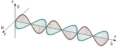
Figure 1. Classical electromagnetic wave, with schematic representation of the orientation of the vectors E, B and .
vector of electromagnetic wave propagation, represented by , can be summarized in the equation
(5)
where:
represents the speed of light in a vacuum [3].
The density of electromagnetic energy U is given by the expression [3]
(6)
while the Poynting vector [3]
(7)
represents the current density of electromagnetic energy. In a flat classical wave, the densities of electric and magnetic energy are equal ( ).
This work develops analogies essentially with the equations related to a wave propagating in a vacuum, in the absence of charges and currents. Maxwell’s equations in these conditions are given in [3]:
(8)
(9)
(10)
(11)
Still from Figure 1, we will represent the unit vectors of the canonical base as follows:
(12)
(13)
(14)
Note that equation
(15)
implies or , that is:
(16)
Also note that , where α is a constant.
But and then:
(17)
Regarding the Poynting vector:
(18)
At the same time:
(19)
(20)
The results (19) and (20) are consistent, and are useful in obtaining and simplifying the results shown in the next sections, that represent the true purpose of this paper.
3. Hypothetical Vector Field Associated with Classical Electromagnetic Wave in a Four-Dimensional Space
Equation (15) can be represented from vector products in four dimensions, as shown in [1] and [2].
Defining the unit vector :
(21)
where . There is then
(22)
with
(23)
It is important to note that (23) is in agreement with the theory:
(24)
COROLLARY: Considering the monochromatic flat wave, the relationship between the magnetic induction vector B, the electric field vector E, and the vector in the direction of propagation of the electromagnetic wave can be represented in the following equation developed for a 4-dimensional space:
(25)
PROOF:
(26)
It is important to note that even here
(27)
which is in agreement with the theory.
PROPOSITION:
PROOF:
(28)
which naturally implies:
(29)
The vector G has the same direction as , being orthogonal to all the vectors of the electromagnetic wave. This can be synthesized by:
(30)
At the same time:
(31)
And also:
(32)
A possible assumption is that the term represents the energy
density associated with the hypothetical field G. One can speak of an energy density of the “electromagnetic wave with the inclusion of the field G”, treated here as a G-electromagnetic wave. Such an energy density would be , and the portion has no effect on the xyz system.
The total “G-electromagnetic energy density” is
(33)
4. Analog of Maxwell’s Equations for the Four-Dimensional Space
In what follows, for simplicity, it is considered:
(34)
where
(35)
In (35) the index h refers to the h-axis, which is orthogonal to the axes of the xyz system, and has the same direction as the unit vector . The following identities will also be used, which can be proved with the development of determinants of order 4 and 3 respectively, from the concept of the analog of the curl vector defined in [2].
(36)
(37)
All developments have essentially the following mathematical characteristics, not speculating possible physical interpretations of the results. The equations related to the divergence of the magnetic and electric fields (10) and (11) are not of particular interest, since their representation in four dimensions would only require the addition of a fourth component. Therefore, developments and demonstrations are focused on analogies with Equations (8) and (9), which involve the curl vector of fields B and E. Using (4):
1) Developing the relationship for E:
(38)
Therefore:
(39)
2) Developing the relationship for B:
(40)
Therefore:
(41)
3) Developing the relationship for G:
(42)
Equation (42) is obvious, since , noting that .
An important result can be obtained by combining Equations (39) and (41). Also note that these results relating fields B and E were obtained from the four-dimensional model.
Differentiating (39) with respect to t, and (41) with respect to z:
(43)
(44)
Noting that and replacing (43) in (44):
(45)
Differentiating (39) with respect to z and (41) with respect to t:
(46)
(47)
Noting that and replacing (47) in (46):
(48)
Equations (45) and (48) show that even in the four-dimensional model, the components of the electric and magnetic fields satisfy the one-dimensional wave equation, with speed of propagation .
5. Results Involving the Hypothetical Vector Field G
Considering the unit vectors and , and relations :
(49)
This equation can be rewritten, showing a direct relationship between fields E and G:
(50)
There is a similar way:
(51)
This equation can be rewritten, showing a direct relationship between fields B and G:
(52)
It is known that . Differentiating this relation separately in relation to t and z:
(53)
(54)
Replacing (53) and (54) in the wave Equation (45):
(55)
As , we have that , and so:
(56)
Noting that by (49) and (50), and because of , and replacing in (56):
(57)
This important result shows that the second member in (55) is zero, and therefore:
(58)
The hypothetical vector field G also satisfies the one-dimensional wave equation, with speed of propagation .
The same result is obtained using the wave Equation (48).
Some more additional results are presented involving the hypothetical vector field G. As previously, all of them result from the product of vectors defined by Equation (1), from the vector analogous to the curl one given by Equation (4), and from the other results obtained in the previous sections:
(59)
(60)
Since , the results above can be written as:
(61)
(62)
Note that the displacement current it is related to also in the model in four dimensions.
Since and , the “energy density” can be written and manipulated as follows:
(63)
In the absence of current and charges, would be simply:
(64)
Writing , it results that:
(65)
This is the local form of the Energy Conservation Law.
6. Conclusions
Through the previously developed concepts regarding vector products in higher dimensions, as well as the use of the vector analogous to the curl vector for a four-dimensional space, it was possible to study the classical electromagnetic wave equations with a focus on a dimensional space larger than three.
In this context, it was shown that the inclusion of a hypothetical vector field G to the electromagnetic wave does not alter the wave representations for fields B and E, known for the IR³ space, at the same time that they are fully equivalent in the IR4 space.
Still in relation to the vector field G, it was possible to show that it meets equations analogous to Maxwell’s equations for the classical electromagnetic wave. Although it was never intended to make physical interpretations for the hypothetical vector field, it was visible that it retains fundamental mathematical properties, such as satisfying the one-dimensional wave equation, presenting an expression for a kind of “energy density” that is consistent with the results already known for the electromagnetic wave, and complies with the energy conservation law.
Conflicts of Interest
The author declares no conflicts of interest regarding the publication of this paper.
Cite this paper
Simal Moreira, L. (2020) On a Hypothetical Vector Field Associated with the Classic Electromagnetic Wave in a Space of Four Dimensions. Journal of Applied Mathematics and Physics, 8, 2836-2845. https://doi.org/10.4236/jamp.2020.812209
References
- 1. Simal Moreira, L. (2013) Geometric Analogy and Products of Vectors in n Dimensions. Advances in Linear Algebra & Matrix Theory, 3, 1-6. https://doi.org/10.4236/alamt.2013.31001
- 2. Simal Moreira, L. (2014) On the Rotation of a Vector Field in a Four-Dimensional Space. Applied Mathematics, 5, 128-136. https://doi.org/10.4236/am.2014.51015
- 3. Nussenzveig, H.M. (2015) Curso de Física Básica Vol 3. 2nd Edition, Blucher, São Paulo.