American Journal of Computational Mathematics
Vol.4 No.3(2014), Article
ID:47196,9
pages
DOI:10.4236/ajcm.2014.43020
Blind Signal Processing in Telecommunication Systems Based on Polynomial Statistics
Oleg Goryachkin, Andrey Berezovskiy
Povolzhskiy State University of Telecommunications and Informatics, Samara, Russia
Email: andrey.berezowskiy@gmail.com
Copyright © 2014 by authors and Scientific Research Publishing Inc.
This work is licensed under the Creative Commons Attribution International License (CC BY).
http://creativecommons.org/licenses/by/4.0/


Received 22 March 2014; revised 23 April 2014; accepted 9 May 2014
ABSTRACT
The tendencies of the contemporary communication systems development are characterized by the increasingly stringent requirements for maximum channel utilization. Considering discrete communication systems in channels with intersymbol interference identification with the use of training signal is the key technology to create various types of equalizers. However, the time (from 20% to 50%) spent on training signal is increasingly attractive resource for upgrading standards TDMA, especially in mobile systems. An alternative method to training signal is blind signal processing.
Keywords:Blind Channel Identification, Polynomial Cumulants, Gröbner Basis

1. Introduction
Blind signal processing is a new technology of digital signal processing which has been developed over the last ten years. The methods and algorithms of blind signal processing can be used not only in application to communication systems, but also in radio astronomy, or to process digital speech, images, radar signals. In general, the problem of blind signal processing can be formulated as digital processing of unknown signals, blurred with unknown linear operator with additive noise.
There are two types of problems that blind signal processing can solve: blind channel identification (unknown impulse response function estimation) and blind equalization (direct useful signal estimation). In both cases only output blurred noisy signal is available for processing. In case of blind identification, impulse response function estimation could be further used to estimate the useful signal, i.e. the first stage of blind equalization.
The problems of blind signal processing presume a wide range of the observed signal models. In case of single input and multiple output (SIMO) the continuous model of the system can be described by the following equation:
 (1)
(1)
where ![]() is the observed signal defined in
is the observed signal defined in ,
,![]() —unknown impulse response function of
—unknown impulse response function of —dimensional channel;
![]() —additive noise (the vector of the stochastic processes as a rule with i.i.d. components);
—additive noise (the vector of the stochastic processes as a rule with i.i.d. components);![]() —unknown useful signal.
—unknown useful signal.
Blind system identification is understood as an ability to restore impulse response function of the system up to a complex factor using only output signal. From the first sight such kind of problem might seem incorrect; nevertheless, it is not the case if blind channel estimation is based on the use of channel structure or the known properties of the input sequence.
At first the blind equalization algorithm for the communication channel in the digital systems with amplitude modulation was suggested by Sato in 1975 [1] . Sato’s algorithm was later generalized by Godard in 1980 [2] for the case of amplitude phase modulation also known as constant modulus algorithm (CMA). In general case the algorithms of this type belong to the class of so-called stochastic gradient algorithms for blind equalization which are built according to the principle of the adaptive equalizer. Error signal of the adaptive equalizer in this case is formed by the nonlinear map of the output signal, the form of which is dependent on the used coding scheme [3] .
Then, another stage of blind signal processing development became the use of higher-order statistics for channel identification, where the input signal is described by non-Gaussian stationary stochastic process [3] [4] . As a rule, these methods help to find the explicit solution for the unknown channel.
A relatively recently understood opportunity to use second-order statistics for multichannel blind identification ![]() has brought the perspective of introducing blind identification techniques to the telecommunication systems significantly closer and induced a whole trend in the recent works [5] [6] , within which a range of high convergence rate identification algorithms is found for today.
has brought the perspective of introducing blind identification techniques to the telecommunication systems significantly closer and induced a whole trend in the recent works [5] [6] , within which a range of high convergence rate identification algorithms is found for today.
The use of second-order statistics for SISO blind identification ![]() is possible for a general case of a non-stationary input signal model and in the particular case of cyclostationary signal. The possibility of blind identification in case of cyclostationary input was shown in [7] , for the inducted cyclostationarity in [8] , and in general case for non-stationary input in [9] .
is possible for a general case of a non-stationary input signal model and in the particular case of cyclostationary signal. The possibility of blind identification in case of cyclostationary input was shown in [7] , for the inducted cyclostationarity in [8] , and in general case for non-stationary input in [9] .
It is necessary to mention that a similar approach to SAR autofocusing using second-order statistics was described independently in [10] [11] .
In this work several blind SISO identification algorithms are introduced, to obtain which the relatively new mathematical apparatus of commutative algebra and algebraic geometry is used.
2. Channel Model
After the signal (1) sampling on the input of the digital signal processing system there is a discrete-time model of the system with a finite input response:
 , (2)
, (2)
where ![]() is discrete useful signal,
is discrete useful signal,![]() —discrete channel impulse response of the length
—discrete channel impulse response of the length ;
;![]() .
.
the input sequence is of finite length, then the formula (2) can be written down as a product of polynomial function of positive degree over a field of complex numbers![]() :
:
![]() (3)
(3)
where 


 . Projection operator
![]() maps the polynomial
maps the polynomial ![]() of
of ![]() degree to polynomial of
degree to polynomial of ![]() degree, zeroing the
degree, zeroing the ![]() least and the
least and the ![]() highest coefficients of the polynomial and the division by
highest coefficients of the polynomial and the division by![]() .
.
In contrast with the use of Z-transform, traditional for digital signal processing, the signals are represented as elements of the polynomial ring over one variable. This kind of representation per se does not give much in the context of our task, since the field of complex numbers is algebraically closed. However, introducing further the notion of polynomial statistics, the task can be transferred to a more meaningful polynomial ring over several variables![]() , where the potentiation of blind identification is higher.
, where the potentiation of blind identification is higher.
3. Polynomial Statistics
The notion of polynomial statistics was used in [12] with an aim to emphasize the difference of the used approach from the methods based on the cumulant analysis and polyspectrums.
Let  be the complex random vector, described by probability density function
![]() , is defined on
, is defined on![]() . Let us call the polynomial moment of
. Let us call the polynomial moment of ![]() order
order ,
,  of a random vector
  polynomial of r variables belonging to the ring
 ![]() over a field of complex numbers formed as:
over a field of complex numbers formed as:
 . (4)
. (4)
Apparently the set of polynomial moments defined that way (4) defines entirely the probability density function and characteristic function of complex random vector formed by evaluation of the random polynomial
![]() at the points
at the points![]() .
.
The polynomial moment of the sum of independent random polynomials is not equal to the sum of polynomial moments of random polynomials, therefore it is more suitable to use the generalized correlation or random polynomials cumulant values.
Let us define the polynomial cumulant of ![]() order,
order,  ,
,  random vector
  as a polynomial of r variables belonging to the ring
![]() :
:
 . (5)
. (5)
4. Channel Identification by Polynomial Statistics
For the system (3) cumulant of the output signal (5) can be written as a polynomial in the ring![]() . Then let us formulate (3) as:
. Then let us formulate (3) as:
 , (6)
, (6)
where 
The equation for cumulants of the input and output of the system can be written down substituting (6) to (5).
 (7)
(7)
Setting different points over 
 , the system
  of polynomial equations will be obtained:
 (8)
(8)
The given system of equations defines the affine variety ![]() in
in  and the corresponding ideal
 ![]() in the polynomial ring
in the polynomial ring![]() .
.
Solving a system (8) may result in two possible cases: 1) the number of solutions is finite and less than
![]() (manifold is zero-dimensional); 2) the number of solutions is infinite.
(manifold is zero-dimensional); 2) the number of solutions is infinite.
Channel identifiability is the necessary and sufficient condition for the zero-dimensionality of the manifold (8).
According to Hilbert’s Nullstellensatz, any ideal of the ring ![]() has a finite number of generator polynomials, forming the basis of ideal [13] . Therefore one of the solutions (8) is to choose the basis polynomials, which would be more suitable for solving the system. Normally for solving such systems Gröbner basis of the ideal
has a finite number of generator polynomials, forming the basis of ideal [13] . Therefore one of the solutions (8) is to choose the basis polynomials, which would be more suitable for solving the system. Normally for solving such systems Gröbner basis of the ideal  is chosen; it consists of polynomials, containing variables successively eliminated
  [13] -[15] . This approach is equivalent to Gaussian elimination. Unfortunately the application of this method is an extremely hard computational problem, and it is not adapted to the inexactly specified coefficients. The more acceptable version of the algorithm is described in [16] .
Another approach is based on Stetter’s theorem [14] . If ![]() is zero-dimensional, then the quotient ring
is zero-dimensional, then the quotient ring ![]() as vector space is isomorphic to a finite-dimensional vector space
as vector space is isomorphic to a finite-dimensional vector space . The space
  is formed by the linear manifold of all monomials
![]() , belonging to the complement of the monomial ideal
, belonging to the complement of the monomial ideal![]() .
.
This fact allows to reduce the problem (8) to the eigenvalues evaluation of the linear operators having special forms, defined on the . Stetter’s theorem, obtained relatively recently (in 1996), is a generalization of the approach to polynomial roots evaluation over one variable using the eigenvalues of Frobenius matrix.
Let ![]() be the linear transformation matrix mapping
be the linear transformation matrix mapping![]() , and for any polynomial
, and for any polynomial  can be found
 ![]() matrix
matrix ![]() with the elements
with the elements![]() ,
,  so that:
 (9).
(9).
Herewith, if ![]() ,
,  are the eigenvalues of the matrix
![]() , and
, and ![]() is one of the
is one of the ![]() solutions of the (8) system of equations, then eigenspace corresponding to nonzero eigenvalue
solutions of the (8) system of equations, then eigenspace corresponding to nonzero eigenvalue ![]()
could be built with the help of the eigenvector .
.
Thus, finding all the different nonzero eigenvalues of a matrix ![]() and the corresponding eigenvectors, we obtain all the solutions of the system of polynomial Equations (8).
and the corresponding eigenvectors, we obtain all the solutions of the system of polynomial Equations (8).
The disadvantage of the given method is the uncertainty of polynomial  choice and the instability of the solution in case of the coefficient perturbation of the system of Equations (8). To overcome the latter disadvantage further regularization is used.
Thus, with the use of polynomial statistics, the solution of the blind identification problem is reduced to the problem of solving the systems of polynomial equations over multiple variables. This is a generalization of another approach based on the use of polyspectrums (so-called higher-order statistics method), well-known within the theory of communication [3] [4] . Accordingly, some common disadvantages of the methods using moments and cumulants are inherent to the proposed method as well. First of all, this has to deal with low convergence rate of the obtained estimations. However, as we will see later, in the framework of the approach we will be able to additionally optimize algorithm parameters. These possibilities are further illustrated with the example of scalar channel blind identification with non-stationary input using second-order statistics.
5. Identification Algorithm Synthesis Based on Second-Order Statistics
Let us write down the second-order polynomial moments equation, corresponding to the system model of the form (7):
 , (10)
where
 (11)
(11)
In particular, if the input signal samples are uncorrelated, have dispersion ![]() and zero expectation, then the corresponding polynomial moments in the input sequence in (11) would look like:
and zero expectation, then the corresponding polynomial moments in the input sequence in (11) would look like:
 (12)
(12)
Setting different points in , corresponding to the values of the (formal) variables
  in
in
(12), we obtain a system of polynomial equations (8), containing the unknown variables . For the identified system the number of solutions is finite and does not exceed
![]() .
.
It is necessary to mention that all polynomials of the system of equations (8) are formed by the monomials of the form![]() . Let us introduce new variables
. Let us introduce new variables![]() , where
, where , so that
![]() , then the system (8) can be written down as a system of linear equations:
, then the system (8) can be written down as a system of linear equations:
 (13)
(13)
where: elements of matrix ,
,  , and components of the vector
![]() ,
, . If the conditions of identifiability are satisfied, then the system of equations
(13) is consistent and the matrix  rank is equal to
 . Then there exists a unique vector
![]() , so that the system (8) is equivalent to the system of polynomial equations having the form of:
, so that the system (8) is equivalent to the system of polynomial equations having the form of:
 (14)
(14)
For the system of Equations (10) it is easy to define the monomials belonging to the complement of the monomial ideal , these are
 . Let
. Let , then the matrix
 ![]() has the form of:
has the form of:
 (15)
(15)
Such matrix has only two nonzero eigenvalues, which correspond to the two solutions of the system (8), differing by constant factor. Let  be the eigenvector corresponding to the nonzero eigenvalue of the matrix
 ![]()
(15), then channel estimation is directly given by vector  components
![]() .
.
As far as the vector ![]() of the system (13) is known with an error, caused by the additive noise and the use of sample covariance matrix of the observed signals, then the solution of the system (13) will contain an error, the value of which is dependent on the signal-to-noise ratio and the number of signal realizations used to estimate the covariance matrix; therefore to solve the system (13) Tikhonov regularization is used.
of the system (13) is known with an error, caused by the additive noise and the use of sample covariance matrix of the observed signals, then the solution of the system (13) will contain an error, the value of which is dependent on the signal-to-noise ratio and the number of signal realizations used to estimate the covariance matrix; therefore to solve the system (13) Tikhonov regularization is used.
6. Simulation
This section shows the results of the simulation of blind identification algorithm based on second order statistics for the case of periodic non-stationary modulation of the useful signal. Relative error of impulse response function was estimated using the formula:
 . (16)
Computer algebra system “Maple” was used in the simulation to evaluate the Gröbner basis.
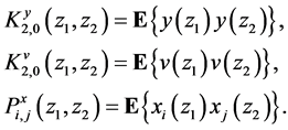
The simulation was ran for the useful signal of white Gaussian noise model with dispersion modulated by a discrete signal. The unknown impulse response function:![]() ; period of the discrete signal used for modulation 10.
; period of the discrete signal used for modulation 10.
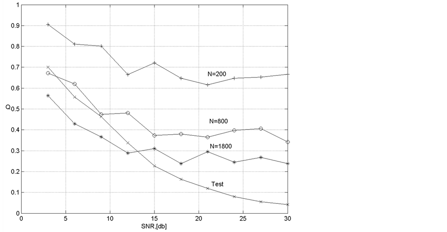
Discrete signal used for modulation was applied in the simulation shown on Figure 1 and Figure 2. For the discrete signal used for modulation on Figure 1 in case of ![]() the results are shown on the Figures 3-5 respectively. Except for the error graph of blind identification algorithm for different length of useful signal all figures show the impulse response function estimation error using the training signal. For the discrete signal used for modulation on Figure 2 the results of the simulation are shown on the Figure 6.
the results are shown on the Figures 3-5 respectively. Except for the error graph of blind identification algorithm for different length of useful signal all figures show the impulse response function estimation error using the training signal. For the discrete signal used for modulation on Figure 2 the results of the simulation are shown on the Figure 6.
The general characteristic of scalar channel statistical identification is the relatively low rate of convergence. However for the discrete signal used for modulation with ![]() (Figure 6) the error is weakly dependent on the length of useful signal, and with the high signal-to-noise ratio could be quite competitive in comparison with the estimation by the training signal already at
(Figure 6) the error is weakly dependent on the length of useful signal, and with the high signal-to-noise ratio could be quite competitive in comparison with the estimation by the training signal already at![]() .
.
One of the works [15] suggests a highly effective blind identification algorithm, which is also based on the use of polynomial statistics; however, it is directly using the opportunities of one-to-one unions factorization of affine variety of the channel and useful signal polynomial cumulants. This algorithm has a higher rate of convergence, however it is more dependent on the level of additive noise.
Discrete signal used for modulation on Figure 2 is characterized by having the constant modulus of the amplitude envelope; it can be used in the systems with phase modulation [8] . If the length of useful signal is more

Figure 1. Type I discrete signal used for modulation.
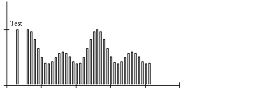
Figure 2. Type II discrete signal used for modulation.

Figure 3. The results in case of A= 2 for the discrete signal used for modulation on Figure 1.
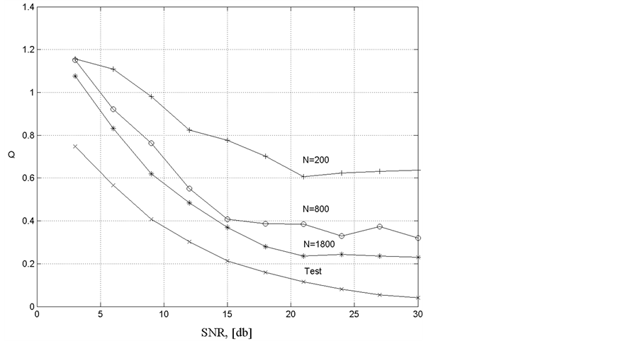
Figure 4. The results in case of A= 4 for the discrete signal used for modulation on Figure 1.
than 2000, then the estimation error becomes less than it is in case of using training signal even with small signal-to-noise ratio.
The error of blind identification algorithm decreases with increasing the length of useful signal and decreasing the period of discrete signal used for modulation.
In addition to objective factors, the error of the algorithm is affected by the formal variables values choice  in
in , used in Equation (12). Furthermore, the use of regularization method in the solution of the system (13) requires the optimal selection of the regularization parameter. During the simulation Monte Carlo method was used to optimize these parameters of the algorithm.

Figure 5. The results in case of A= 10 for the discrete signal used for modulation on Figure 1.
7. Conclusions
Thus, the proposed approach to the synthesis of the blind identification algorithms based on the polynomial statistics allows synthesizing with the same methodology different blind identification algorithms for scalar channels with stationary and non-stationary input and different input symbols distributions. In contrast with polyspectrums approach, in this case the uncertainty of the cumulant functions set choice might be reduced at least in the relation to the procedures of the algorithm synthesis. It is necessary to mention that this approach can be generalized for the case of the vector channel as well.
In the scalar channel, that is the channel with single input and single output (SISO) blind identification algorithms, as a rule, require certain data sample collected on the output for the channel estimation. Generally, for the unspecified identification method and channel properties, to obtain blind estimation in the scalar channel the useful signal is required; the length of it is usually two orders of magnitude greater than the channel length. Herewith the quality of the estimation is close to the estimation by training signal.
It is necessary to mention that solving a number of practical problems the use of training signal is impossible or undesirable, and the use of blind identification is the only option. This might include the problems of signals intelligence, unauthorized access to transmitted information, asynchronous data exchange etc.
The effectiveness is different in case of using blind estimation in vector channels, i.e. channels with single input and multiple output (SIMO) [6] . SIMO model is used to describe the diversity reception in space or in time. The conditions of identifiability of the vector channel can be formulated within the framework of deterministic model, i.e. blind identification is done using one realization in the same way as with using the training signal. Herewith channel length to useful signal ratio is approximately of one order of magnitude which allows using these technologies in the fast-fading channels.
Generally, blind signal processing is an intensively developing field of DSP and this article particularly opens a wide range of opportunities for further research.
References
- Sato, Y. (1975) A Method of Self-Recovering Equalization for Multilevel Amplitude-Modulation Systems. IEEE Transactions on Communications, 23, 679-682. http://dx.doi.org/10.1109/TCOM.1975.1092854
- Godard, D.N. (1980) Self-Recovering Equalization and Carrier Tracking in Two Dimensional Data Communication Systems. IEEE Transactions on Communications, 28, 1867-1875. http://dx.doi.org/10.1109/TCOM.1980.1094608
- Proakis, J. (2000) Digital Communications. McGraw-Hill Science/Engineering/Math, New York.
- Nikias, H.L. and Raguver, M.R. (1987) Bispektral’noe ocenivanie primenitel’no k cifrovoj obrabotke signalov. TIIJeR, 75, 5-30.
- Liu, H., Xu, G., Tong, L. and Kailath, T. (1996) Recent Developments in Blind Channel Equalization: From Cyclostationarity to Subspaces. Signal Processing, 50, 82-99. http://dx.doi.org/10.1016/0165-1684(96)00013-8
- Tong, L. and Perreau, S. (1998) Blind Channel Estimation: From Subspace to Maximum Likelihood Methods. IEEE Proceedings, 86, 1951-1968.
- Tong, L., Xu, G. and Kailath, T. (1991) A New Approach to Blind Identification and Equalization of Multipath Channels. Proceedings of the 25th Asilomar Conference on Signals, Systems and Computers, 4-6 November 1991, Pacific Grove, 856-860.
- Serpedin, E. and Giannakis, G.B. (1997) Blind Channel Identification and Equalization with Modulation Inducted Cyclostationarity. IEEE Transactions on Signal Processing, 46, 1930-1944.
- Goriachkin, O.V. and Klovsky, D.D. (2001) Blind Channel Identification with Non-Stationary Input Processes. Proceedings of World Multiconference on Systemics, Cybernetics and Informatics, 22-25 July 2001, Orlando, 386-388.
- Gorjachkin, O.V. (1996) Avtomaticheskaja fokusirovka izobrazhenij v radiolokatore s sintezirovannoj aperturoj. Analiz signalov i sistem svjazi: Sb. nauch. tr. ucheb. zaved. Svjazi, SPbGUT, SPb, No. 161, 128-134.
- Goriachkin, О.V. and Klovsky, D.D. (1996) Non-parametrical Focusing in the SAR. Proceedings European Conference on Synthetic Aperture Radar, 26-28 March 1996, Konigswinter, 551.
- Gorjachkin, O.V. (2002) Polinomial’nye predstavlenija i slepaja identifikacija system. Fizika volnovyh processov i radiotehnicheskie sistemy, No. 4, 53-60.
- Cox, D., Little, J. and O’Shea, D. (1992) Ideals, Varieties, and Algorithms: An Introduction to Computational Algebraic Geometry and Commutative Algebra. Springer, New York.
- Stetter, H.J. (1995) Matrix Eigenproblems at the Heart of Polynomial System Solving. SIGSAM Bulletin, 30, 22-25.
- Gorjachkin, O.V. (2003) Algoritm slepoj identifikacii, osnovannyj na analize affinnyh mnogoobrazij nezavisimosti polinomial’nyh kumuljantov sluchajnyh posledovatel’nostej. Trudy 58-j nauchnoj sessii RNTORJeS im. A.S. Popova-g. Moskva, 14-15 maja, t.1, C.67-69.
- Gorjachkin, O.V. (2003) Algoritm slepoj identifikacii nestacionarnogo po vhodu kanala svjazi po polinomial'nym statistikam vtorogo porjadka. Sbornik dokladov mezhdunarodnoj nauchno-tehnicheskoj konferencii, Radio i volokonno-opticheskaja svjaz, lokacija i navigacija.-g. Voronezh, t.1, C.274-279.