Journal of Modern Physics
Vol.3 No.2(2012), Article ID:17676,16 pages DOI:10.4236/jmp.2012.32018
Mechanisms of Proton-Proton Inelastic Cross-Section Growth in Multi-Peripheral Model within the Framework of Perturbation Theory. Part 3
1Department of Theoretical and Experimental Nuclear Physics, Odessa National Polytechnic University, Odessa, Ukraine
2Department of Experimental Particle Physics, Jožef Stefan Institute, Ljubljana, Slovenia
3Department of Mathematics, Bielefeld University, Bielefeld, Germany
Email: *siiis@te.net.ua
Received July 28, 2011; revised September 5, 2011; accepted October 26, 2011
Keywords: Inelastic Scattering Cross-Section; Total Scattering Cross-Section; Laplace Method; Virtuality; Multi-Peripheral Model; Regge Theory
ABSTRACT
We develop a new method for taking into account the interference contributions to proton-proton inelastic cross-section within the framework of the simplest multi-peripheral model based on the self-interacting scalar φ3 field theory, using Laplace’s method for calculation of each interference contribution. We do not know any works that adopted the interference contributions for inelastic processes. This is due to the generally adopted assumption that the main contribution to the integrals expressing the cross section makes multi-Regge domains with its characteristic strong ordering of secondary particles by rapidity. However, in this work, we find what kind of space domains makes a major contribution to the integral and these space domains are not multi-Regge. We demonstrated that because these interference contributions are significant, so they cannot be limited by a small part of them. With the help of the approximate replacement the sum of a huge number of these contributions by the integral were calculated partial cross sections for such numbers of secondary particles for which direct calculation would be impossible. The offered model qualitative agrees with experimental dependence of total scattering cross-section on energy  with a characteristic minimum in the range
  ≈ 10 GeV. However, quantitative agreement was not achieved; we assume that due to the fact that we have examined the simplest diagrams of
  theory.
1. Introduction
This paper is the sequel to [1,2], where to calculate protonproton scattering partial cross-sections within the framework of multi-peripheral model the Laplace method was applied.
The inelastic scattering amplitude with production of a specified multiplicity of secondary particles, in framework of the multi-peripheral model can be represented as a sum of diagrams demonstrated on Figure 1.
To calculate the partial cross-section  is necessary to evaluate an integral of the squared modulus of a sum of contributions shown in Figure 1. After simple transformations [2], the expression for the partial cross-section can be represented as a sum of “cut” diagrams in Figure 2. We call summands entering into the sum Figure 2 the interference contributions. Approximate calculation of their sum is the purpose of this paper.
At present time the inelastic scattering processes are considered without the interference contributions [3,4]. This due to the generally adopted assumption that the main contribution to the integrals expressing an inelastic processes makes multi-Regge domains [3-6] with its characteristic strong ordering of secondary particles by rapidity. This means that the rapidity of neighboring particles on the “comb” should be different from each other by a large value. Thus the amplitude of the right-hand and left-hand parts of the diagram on Figure 2 for different orders of connecting lines would be significantly different from zero to almost non-overlapping regions of phase space and integral of their product would be a small quantity.
However, as it was shown in [1] near the threshold of the  particles production at the maximum point of the

Figure 1. Diagram representation of an inelastic scattering amplitude when the n secondary particles are formed. Here P1 and P2 are the four-momenta of primary particles before scattering; P3 and P4 are the four-momenta of primary particles after scattering; 

 are the fourmomenta of secondary particles. Symbol
  denote a sum over all permutations of indices i1 = 1, i2 = 2,
  in = n. Plotting of diagrams of the “comb” type.
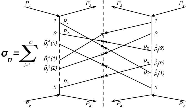
Figure 2. Representation of the partial cross-section as a sum of “cut” diagrams. The order of joining of lines with four-momenta pk from the left-hand side of the cut is as following: the line with p1 is joined to the first vertex, the lines with p2 is joined to the second vertex, etc. The order of joining of lines from the right side of cut corresponds to one of the n! possible permutations of the set of numbers 1, 2,  n. Where
 , k = 1, 2,
  n denote the number into which a number k goes due to permutation
 . An integration is performed over the four-momenta pk for all “cut lines” taking into account the energy-momentum conservation law and mass shell condition for each of pk.
scattering amplitude Figure 1 difference between neighboring particle’s of rapidities is close to zero and at higher energies increases logarithmically with energy  growth. This difference has factor 1/(n + 1), so for high numbers of secondary particles it increases slowly with energy. Moreover, even if each of interference terms is insignificant, all of them are positive and a huge amount n! of them not only makes it impossible to discard them, but also leads to the conclusion that the contribution of a “ladder” diagram Figure 2, which is usually only taken into account, is negligibly small compared with the sum of the remaining interference terms. This was shown in [2]. For the relatively small number of secondary particles (
 ) we are able to calculate all the interference contributions in the direct way without any approximations.
Further in this paper we will demonstrate method for approximate calculation of the sum of the interference contributions for large numbers of secondary particles, when direct numerical calculation is not feasible.
2. Method Description
Using the Laplace’s method we have found [1,2] the mechanism of partial cross-section growth, which was not taken into account in the previously known variants of multi-peripheral model. This mechanism may be responsible for the experimentally observed increase of hadronhadron total cross-section. However, in this approach based on the Laplace’s method, it was found out that the calculation of partial cross-sections in the multi-peripheral model can be limited just to contributions from the “cut ladder diagram”. Because for any number of the secondary particles n there is the wide range of energies , where such contribution is negligibly small compared. Because for any number of the secondary particles n there is the wide range of energies
 , where such contribution is negligibly small compared to the sum of n! positive interference contributions. At the same time, as we will demonstrated further, the allowance for the interference contributions results in the appearance of multipliers in expression for the partial cross-section, which are decrease with the energy
  rise (see below Equation (7)). Thereupon the question arises: “Will the sum of partial cross-sections increase with energy rise if we take interference summands into account?
As shown in [1], each term in sum shown in Figure 1 with accuracy up to the fixed factor is a function with real and positive values, which has a constrained maximum if its arguments satisfy the mass-shell conditions and energy-momentum conservation law. Therefore, in the c.m.s. of initial particles function corresponding to the left-hand part of cut diagram in Figure 2 can be rewritten in the neighborhood of maximum point in the form [1,2].
 (1)
(1)
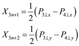
where  is the column composed of 3n + 2 independent variables, on which the scattering amplitude depends after consideration of mass-shell conditions and energymomentum conservation law; the first n components of column are the rapidities of secondary particles; the next n components are the x components of transversal momenta of secondary particles (it is supposed that the reference system is chosen so that z-axis is directed in the line of the three-dimensional momentum P1 of initial particle in Figure 1), the y-components of secondary particle transversal momenta and the two last variables are the antisymmetric combinations of particle transversal momenta P3 and P4, i.e.,
We denote the column of the values of variables in a maximum point through  and a matrix with the elements.
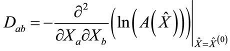 (2)
(2)
where
 (3)
(3)
are the coefficients of the Taylor series expansion of amplitude logarithm in the neighborhood of maximum point. As it was shown in [1], if we do our computations in the c.m.s. of initial particles, the maximum is reached when transversal momenta is zero and secondary particle rapidities are close to numbers that formed an arithmetic progression.
If we denote the difference of this progression through 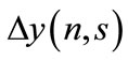 and the value of particle’s rapidity to which the line attached to the k-th vertex of diagram in Figure 1 corresponds, through
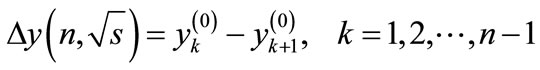 (4)
(4)
we get [1]:
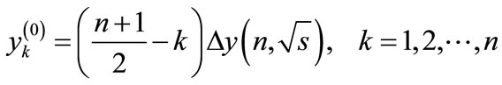 (5)
(5)
The form of the function  has been discussed in [1]. For further consideration, it is important that it is a slowly increasing function on s and decreasing function on the number n of the secondary particles and vanishes when s is equal to the threshold of n particle production. Thus, the column
  contains only the first nonzero n rapidity components, which are defined by Equation (5).
The following expression corresponds to the right-hand part of cut diagram in Figure 2:
 (6)
(6)
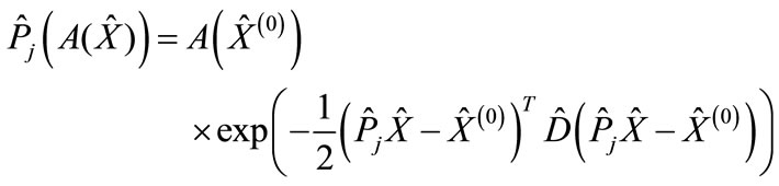
The interference contribution corresponding to whole “cut” diagram, which correlates with the j-th summand in Figure 2, is proportional to an integral of the product of functions Equation (1) and Equation (6) over all variables. Denoting an interference summand corresponding to the permutation  through
  and calculating its Gaussian integral (at the same time, other multipliers besides the squared modulus of scattering amplitude in an integrand are approximately replaced by their values at the maximum point [2]), we get
 (7)
(7)
where we use the following notations:
 (8a)
(8a)
 (8b)
(8b)
 (8c)
(8c)
 (8d)
(8d)
 is the mass of initial particle, which is made dimensionless by the mass of secondary particle (it is supposed that the energy
  is also made dimensionless by the mass of the secondary particle).
Note, that here and in the following sections we will use the “prime” sign in ours notation to indicate that we use a dimensionless quantity that characterized the dependence of the cross-sections on energy, but not their absolute values.
The value of amplitude at the maximum point  increases with the
  growth due to mechanism of virtuality reduction [1]. However, the distance
  between maximum points of “cut” diagram also increases with the
  growth. Therefore, the exponential factor entering in Equation (7) can decrease with energy growth. This makes considered above question. How competition of these two multipliers will result on the dependence of the sum of partial cross-sections on
 ?
?
Thus, each interference contribution can be computed numerically. However due to the huge number of contributions and large number of secondary particles n the direct numerical calculation of the sum of interference terms in Figure 2 is impossible. We can avoid this difficulty in the following way. The maximum in the right part of cut diagram in Figure 2 is attained at .
.
In other words, a maximum of function, which is associated with the right-hand part of cut diagram, can be obtained from a maximum of function, which maps with the left-hand part of cut diagram, by the rearrangement of arguments. Then the value of each interference contribution is determined by the distance between points of maximum in the right-hand and left-hand part of cut diagram as well as by the relative position of these maximum points, since in different directions contributions to scattering amplitude fall off with distance from point of maximum, in general, with different rate, and also by the relative position of proper directions of the matrices  and
and . In other words, multiplying Gaussian functions corresponding to the right-hand and to the left-hand part of interference diagrams in Figure 2 each time we will obtain as a result Gaussian function, which has the proper value at the maximum point (which we call the “height” of the maximum) and the proper multidimensional volume cutout by resulting Gaussian function from an integration domain (which we call the “width” of the maximum).
We assume that summands in Figure 2 are arranged in ascending order of the distance between the maximum points in the right-hand part and left-hand part of cut diagram (we denote this distance through r) so that “cut” diagram with the initial attachment of lines to the righthand part of diagram corresponds to j = 1. In other words, the line of secondary particle with the four-momentum pi is attached to the i-th top in the right-hand part of cut diagram in Figure 2. As follows from Equation (7), the interference contributions exponentially decrease with the r2 growth. However, in spite of this the interference contributions do not become negligible due to their huge number, which, as discussed below, are increases very rapidly with r2 growth. The value of r2 is proportional to the square of magnitude , which, as was noted above, is zero on the threshold of n particle production and slowly increases with distance from this threshold. Therefore, for each number n there is the fairly wide range of energies close to the threshold, in which the sharpness of decrease of the interference contributions with the r2 increase is small in the sense that it is less important factor than the increase in their number. At such energies, which we call “low”, the partial cross-section
  is determined by the sum of huge number of small interfereence contributions. When the magnitude
 is increased with the further growth of energy
 , the decrease rate of interference contributions increases, while the growth rate of their number with the r2 increase does not change with energy. At such energies, which we call “high”, the main contribution to the partial cross-section is made by the relatively small number of interference terms corresponding to the small r2, which can be calculated by Equation (7). If we compose the n-dimensional vector (we denote it through
  from the particle rapidities Equation (5), which constrainedly maximizes the function associated with the diagram with the initial arrangement of momenta in Figure 2, vectors maximizing the functions with another momentum arrangement will differ from the initial vector only by the permutation of components, i.e., these vectors have the same length. Consider two such n-dimensional vectors, one of which corresponds to the initial arrangement, and another to some permutation, then in the n-dimensional space it is possible to “pull on” a two-dimensional plane on them (as a set of their various linear combinations), where two-dimensional geometry takes place. Therefore, the distance r will be determined by cosine of an angle between the considered equal on length n-dimensional rapidity vectors in the two dimensional plane, “pulled”on them. An angle corresponding to the
  permutation we designate through
 ,
, .
.
Thus, each of the terms in the sum Figure 2 can be uniquely matched to its angle . At the same time the variable
  is more handy for consideration than an angle
 Using Equation (5), can be shown that the variable z can take discrete set of values:
 (9)
(9)
Note that although the relation Equation (5) for the rapidities of secondary particles is satisfied with high accuracy at the maximum point, it is still approximate. This means that those contributions, to which matched one and the same value of variable z in Equation (5), in fact, matched a slightly different from each other values of z.
Consequently, to such contributions correspond a similar but unequal to each other distances between maximum points in a “cut” diagram. In addition, this distance, as was discussed above, is not a unique factor affecting to the value of interference contribution. Therefore, if each interference contribution is associated with the value of variable z by the approximation Equation (5), it appears, that the different values of interference contributions correspond to the one and the same value of  (see Figure 3).
Thus, while each contribution is associated to some value of variable z in the approximation Equation (5), the value of contribution is not the unique function of z. However, the sum expressing the partial cross-section  can be written in the following way
 (10)
(10)
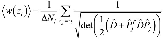
where  the number of summands to which the value
  is corresponds in the approximation Equation (5). The average value of all interference contributions in Equation (10) is already the unique function of
 . Therefore, we introduce notation
 (a)
(a)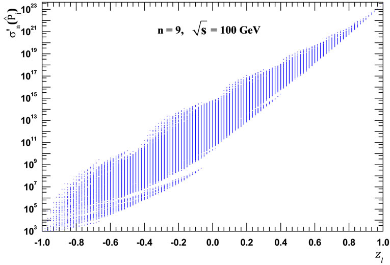 (b)
(b)
Figure 3. The interference contributions dependence on  at
at  = 100 GeV: (a) n = 8; (b) n = 9. Here and in subsequent figures the interference contributions divided by the common multiplier
 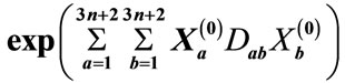 are indicated on the y-axis. Obviously, that to the one value of
  correspond a lot of different contributions, as well as that the average values of the logarithms of these contributions are placed approximately on a straight line (see below Equation (25) and Figure 4).
 (11)
(11)
where  is some function, whose form at “low” energies can be determined from the following considerations.
For any multiplicity n when the values of parameter l in Equation (9) are small and when number of corresponding interference contributions is relatively small, we can directly calculate these elements and their sum. Denote the maximum value l, for which all interference contributions are calculated through l0. In particular, in this paper we managed to calculate the interference contributions up to l0 = 6. Partial cross-section can be written as
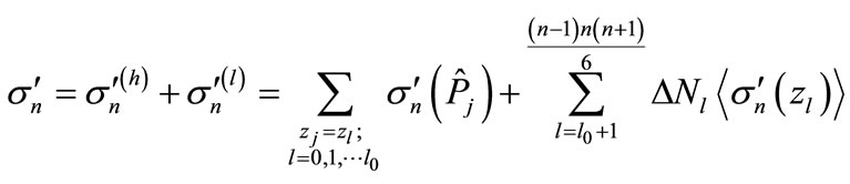 (12)
(12)
where  is the sum of contributions sufficient at “high” energies, and
  is the sum of contributions sufficient at “low” energies. Thus, the difficulties in the calculations of the huge number of interference contributions mainly relates to the range of “low” energies and can be reduced to the approximate calculation of
  and
and .
.
3. The Approximate Calculation of 
As follows from Equation (7), the exponential factor exerts the most significant effect on the dependence of  on
on . Note that the expression
  entering into the exponent in Equation (7) depends only on those matrix
  components, which are at the intersection of the first n rows and first n columns, since all column
  components starting with
  are zerobecause they are the particle momentum transverse components at the maximum point. If we denote the matrix composed of elements located at the intersection of the first n rows and first n columns of the matrix
  through
  and a matrix, which is obtained from the matrix
  in analogy, through
 , we have
 (13)
(13)
The matrices  and
and  have one and the same eigenvalues, but they correspond to different eigenvectors. We denote the normalized to unit eigenvector corresponding to the minimal eigenvalue of matrix
 through
  and the eigenvalue itself —through
 . This implies
 (14)
(14)
Since the minimum eigenvalue of matrix  is equal to the minimum values of quadratic form
  for the unit vectors
 , the magnitude
  is not lessthan the minimum eigenvalue of matrix
 . By analogy the magnitude
  is not less than the minimum eigenvalue of matrix
 , which coincides with the minimal eigenvalue of matrix
  and is reciprocal of the maximum eigenvalue of matrix
  denoted through
 . Thus,
 . From this it follows that, the maximum eigenvalue of matrix
 does not exceed
 . By analogy we obtain that the minimum eigenvalue of matrix
 is no smaller than
 , where
  is the minimum eigenvalue of matrix
 . Thus, an interval enclosing the eigenvalues of matrix
  is, at least, twice smaller than an interval enclosing the eigenvalues of matrix
 . We can demonstrate that at approximation of an equal denominators [1] the value of
  can be estimated in the following way
 (15)
(15)
i.e., an interval enclosing the eigenvalues of matrix  at any energies and number of particles is less than unitywhereas at the considerable values of
 , i.e. at a distance from the threshold, this interval is much less than unity.
Therefore, if we reduce matrix  to diagonal form, it will be close to a matrix multiple of unit matrix. If we represent this matrix in the form
 (16)
(16)
where  is unit matrix, the eigenvalues of the traceless matrix
  will be small. Then
 (17)
(17)
where  are the eigenvalues of matrix
 is the transformation matrix to the basis composed from the eigenvectors of matrix
  (the summation over repeated indices is supposed). The second term in this sum is small in comparison with the first one due to the smallness of eigenvalues
  as well as due to their different signs (since the trace of matrix
  is zero, the different terms over k partially compensate each other). Therefore, we can adopt the following approximation:
 (18)
(18)
To approximately calculate the trace of matrix  we select the spherically symmetric part of matrix
  representing it in the form
 (19)
(19)
The results of numeral calculation of the eigenvalues of matrix  (which are denoted through

 ) are shown in Table 1. It is obvious that most eigenvalues are close between themselves with the exception of a few eigenvalues, which are substantially smaller. Therefore, these smallest eigenvalues have the highest absolute value of deviations from mean eigenvalue
 . Since all the eigenvalues of matrix
  are positive, which means that their deviation from average value is less than this average in absolute value (see Table 1).
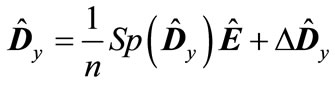
Note that the matrix  can be represented in the following form:
 (20)
(20)
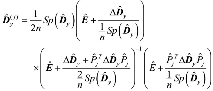
by analogy we can conclude that the minimum eigenvalue of matrix
 (21)
(21)
(which is maximum in absolute value, see Table 1) is greater than the doubled minimum eigenvalue of matrix . This means that all the eigenvalues of matrix
 are less than unity in absolute value. It applies equally to the eigenvalues of matrices
  and
and . Therefore, we can represent the matrix
  as the expansion in powers of
 .Since matrix
  is traceless by definition, then a nonzero contribution to
  in addition to the term term of “zero” order
  can give terms starting with the second-order. As it follows from Table 1, the maximum in absolute value eigenvalue of matrix
 increases with the energy growth. Thereforewe can expect that at “low” energies higher-order terms will make negligibly small contributions. In such an ap-
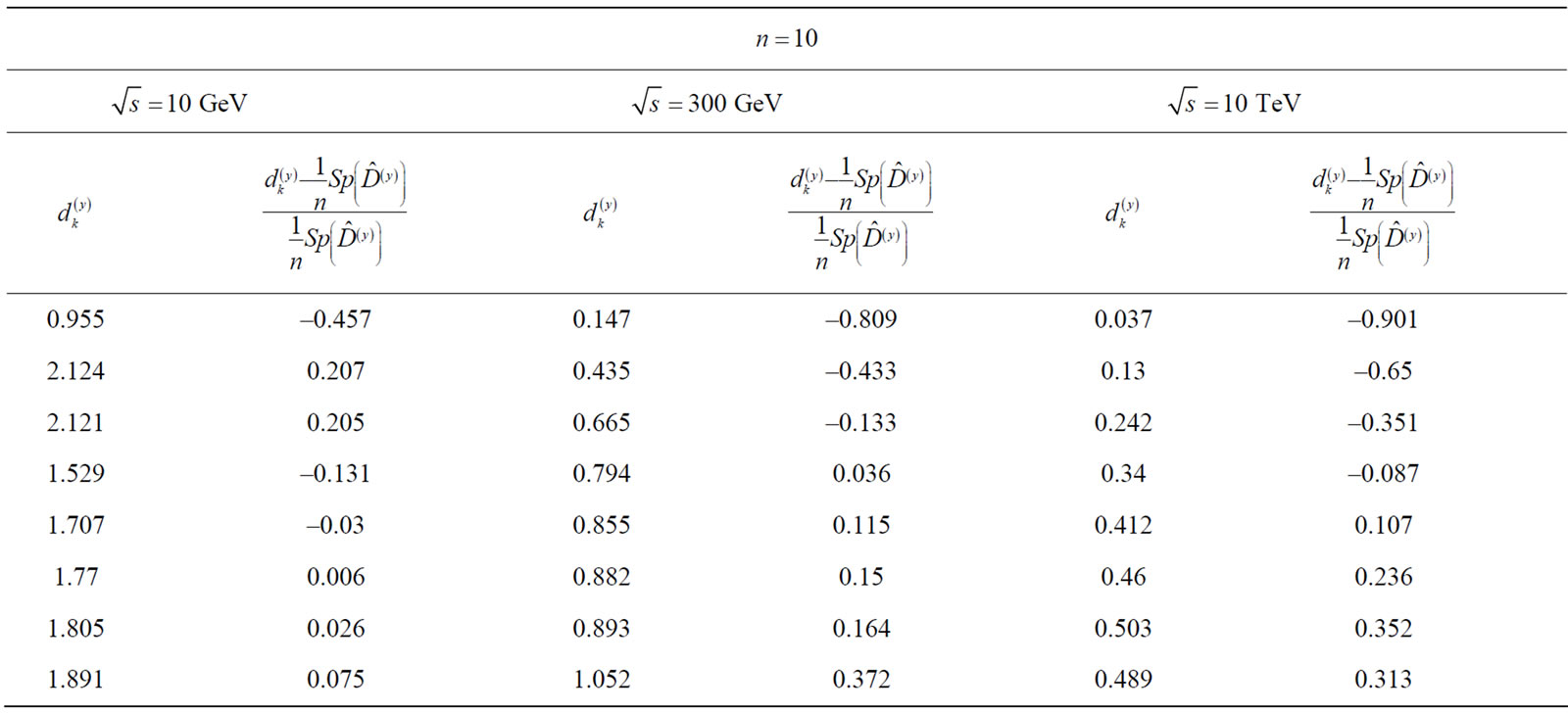

Table 1. Results of numerical calculations of the eigenvalues of matrix .
.
proximation we have:
 (22)
(22)
Let Equation (7) is taken in place of Equation (11) in approximation Equation (22), then we have
 , (23)
Let us introduce the following notation
 . (24)
If we assume that multiplier  is weakly dependent on
 , we obtain
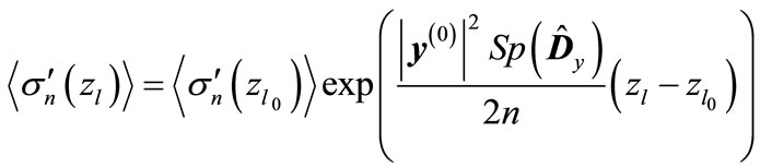 (25)
(25)
where  is the minimum value of
  for which can be numerically calculated all interference contributions. Therefore, the magnitude
  can be directly calculated numerically. The results of numerical calculation of
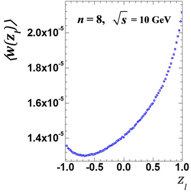
 over all interference contributions in comparison with the results obtained by Equation (24) are demonstrated on Figure 4, it follows that such an approximation is acceptable at “low” energies.
Results shown in Figure 4 confirm also our assumption that  weakly depends on
 . To analyze this dependence we turn to Figure 5. It is obvious, that the magnitude
  takes small values at “low” energies.
 (a)
(a)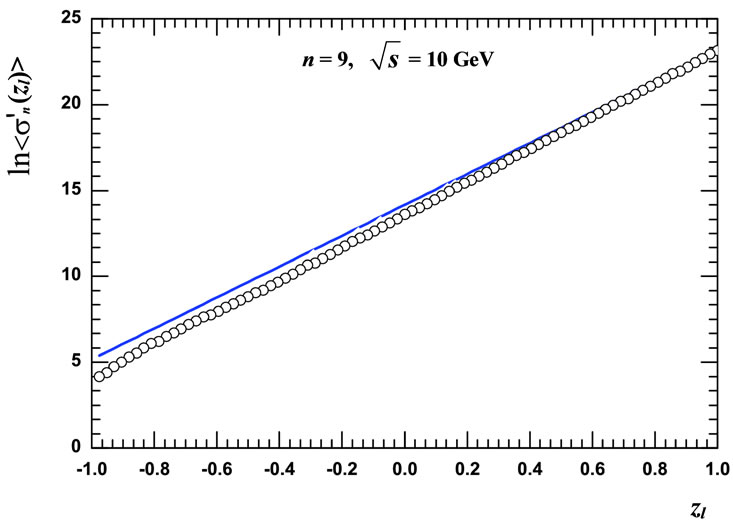 (b)
(b)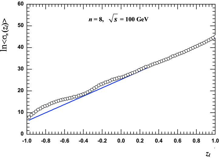 (c)
(c) (d)
(d)
Figure 4. Two results of  evolution by it a direct numerical calculation with consideration of all interference contributions (circles) and by it approximation Equation (24) (straight line) at n = 8,
  = 10 GeV (a); n = 9,
  = 10 GeV (b); n = 8,
  = 100 GeV (c); n = 9,
  = 100 GeV (d).
 (a)
(a)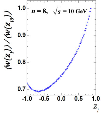 (b)
(b)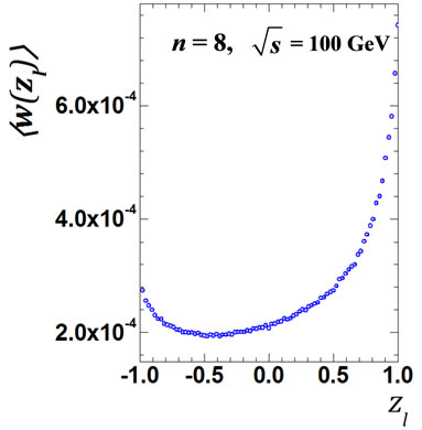 (c)
(c)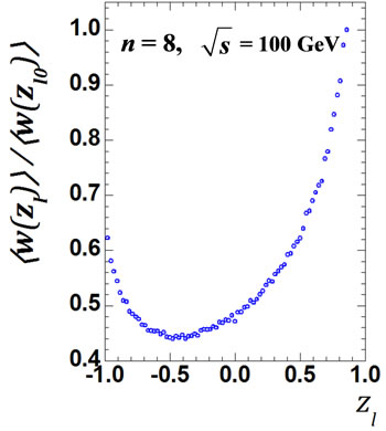 (d)
(d)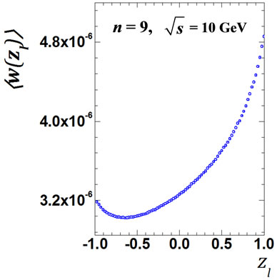 (e)
(e)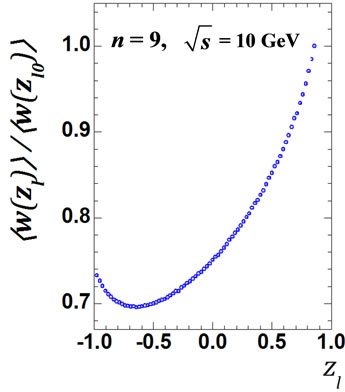 (f)
(f)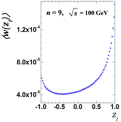 (g)
(g)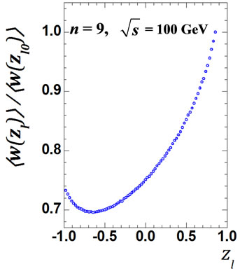 (h)
(h)
Figure 5. The values of  obtained by direct calculation values Equation (24) for all interference contributions for n = 8 and n = 9 at
 = 10 GeV (a), (e) accordingly; for the same number n, but at
  = 100 GeV (c), (g) and the ratio
  for n = 8 and n = 9 at
  = 10 GeV (b), (f);
  = 100 GeV (d), (h).
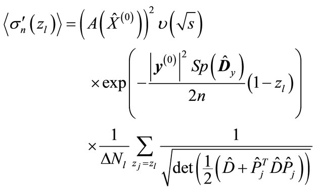
This means that
 (26)
(26)
takes large values at the same energies. Indeed, as it follows from the expression for the matrix , Equation (26) tends to infinity on the threshold of n particle production, and this means that at threshold the volume of phase space with n particles production in the inelastic process is equal to zero.
Because of symmetry with respect to direction inversion in a plane of transversal momenta the mixed second derivatives with respect to rapidities and transversal momentum components are zeros. As a consequence, the determinant Equation (26) is equal to the product of the three determinants, first of which is composed from second derivatives with respect to rapidities, the second is composed from the second derivatives with respect to the transversal momentum x-components and the third one is composed from derivatives with respect to the transversal momentum y-components. All the three factors tend to infinity at the threshold energy. As it follows from a numerical calculation, a matrix determinant composed from the second derivatives with respect to rapidities reduced quite rapidly with energy growth. Matrix determinants composed from the second derivatives with respect to transversal momentum components also reduced, but in a wide energy range, they remain quite large. Therefore, the value of Equation (26) is great at all . Since the function
  varies slightly at the great values of argument, the function
  weakly depends on
 .
.
To estimate roughly the function  we can replace it by the Taylor expansion taking into account just linear contributions. The expansion coefficients are found by the calculating of
  for
for  close to 1 and (−1). In these cases the values of
 (27)
(27)
were obtained directly for all proper interference contributions, and after that we obtain the values of  by averaging using Equation (24).
The values in Figure 5 have been obtained by the direct calculation of
 (28)
(28)
with consideration of all interference contributions at different .
.
So, we have the following expression instead of Equation (25)
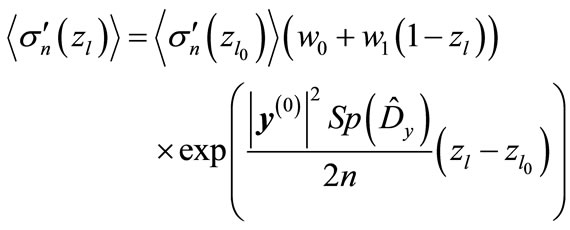 (29)
(29)
where the coefficients  and
and  are found by above mentioned method.
4. Approximate Calculation of the  Values
Let us turn to the new variables
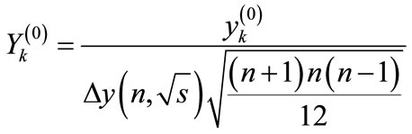 (30)
(30)
where  are determined by Equation (5),

 are considered as the components of vector
 , which, as it follows from Equation (30) is of unit length.
Thus, the angle  between the vector
 and vector
  obtained by the permutation of corresponding components is the same as the angle between the vector
 and vector
 . Moreover, as it follows from Equation (5)
 (31)
(31)
It follows that all vectors  are orthogonal to vector
 (32)
(32)
Therefore, considering vectors  as the elements of n-dimensional Euclidean space, which we de note through
 , then the ends of all vectors
  are lie on the unit sphere embedded into the
  -dimensional subspace of
 . We denote this sphere through
  and shape formed by the set of points in which the ends of vectors
  (
( ,
, ) come, denote through
 . In particular, when
  the sphere
  and figure
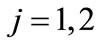
  graphically look like in Figure 6.
We examine some geometrical properties of figure  at arbitrary n. If we apply the permutation transformation component to all vectors in the n-dimensional space, where the vectors
  are primordially defined, the examined
  -dimensional subspace as well as a sphere
  and figure
  go into themselves. As it follows from the group properties of permutation group, the each point of figure
  can be obtained from any other point by some transformation
 . This means that the configuration of the points of figure
  relative to each of these points must be identical, that can be clearly seen in Figure 7(a).
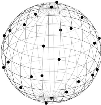
Figure 6. A sphere S2 and figure F4!, which is demonstrated by points. Basis in the four-dimensional space is chosen so that the one of vectors coincides with the vector  and the three basis vectors of three-dimensional subspace, into which depicted sphere is embedded, are perpendicular to e4.
 (a)
(a)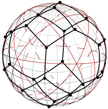 (b)
(b)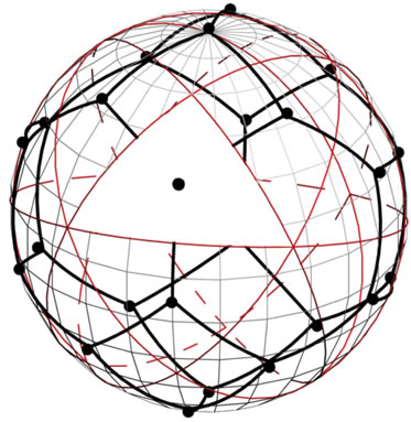 (c)
(c)
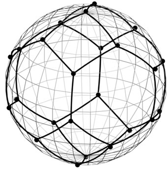
Figure 7. The partition of sphere S2 by shortest arcs joining the points of figure F4! into the two “hexagonal” and one “tetragonal” regions (a); (b) areas, which is located on the borders of 4 or 6 points belonging to figure F4! can be divided between those points into figures of equal area; (c) whole sphere S2 is divided into figures of equal area, each of which contains the one point of figure F4! one of these shapes are painted in white.
As it follows from Equation (31), besides the end of each vector  a figure
  contains also the end of vector
 , i.e., a figure
 has a center of symmetry, which coincides with the center of sphere
 . In this case, if we using point of
  form path from the point
  to the point
 , then it will be simultaneously formed a centro-symmetrical path, that leads from
  to
to  of figure
 .
.
Joining these paths we will obtain the closed path, which “girdles” the sphere . If we assume that there is such a “girdling” path, inside of which are concentrated all points of figure
 , we would find that the figure
  has a “boundary” and “internal” points, that would contradict the fact that spacing of all points relative to each point of the
  should be the same. In other words, the points of figure
  must “crawl away” all over the sphere
  and cannot be concentrated on some area of the sphere.
If we consider a vector , then closest to it are the vectors corresponding to permutations

 defined by the following relation
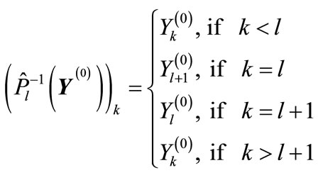 (33)
(33)
The type of “cut” diagrams corresponding to such permutations is shown on Figure 8. At the same time, all the components of vector , except the l-th and l + 1, are zero, whereas these two components take on the least values in modulus
 and
and , respectively.
Thus, we can conclude that the each point of figure  has
has  nearest neighboring points, which lying at distance of from it:
 (34)
(34)
Connecting the each point of figure  with its
  nearest neighbors’ points by shortest arc thereby we divide the sphere
  into closed regions as is shown in Figure 7(a). Indeed, let us choose the some point A0 of figure
  and will move from it to the nearest point A1 along a shortest arc, then we move from the point A1 to the nearest point A2 etc. At the same time, motion in a backward direction is prohibited. Thus, there are
  paths going out from each point, and
  paths are allowed at each step. But since figure
  has the finite number of points at some step we will surely come back to the point A0.
Moreover, since shortest arcs joining two nearest points are subtended by equal chords  in length (see Equation (34)), this arcs are of the same length. Let us consider any two neighboring points
  and
and  of figure
 . Under any transformation
  the shortest arc, which joins the points
  and
and , and an arc joining the points
  and
and  are of the same length.
This means that the boundaries of closed regions formed by shortest arcs, which join neighboring points, replaced into one another under any transformation . It follows that, if we examine closed areas which include any point of figure
 , then the adjacent areas to all points of this figure will have the same “area”.
There is one more requirement, to which the areas obtained by partition of the sphere  must satisfy: they must not overlap, i.e., these regions do not have common internal points. Indeed, otherwise, at least any two of the examined arcs would intersect in some internal point of these arcs. As it follows from Equation (34), when n is large the value of
  is small. This means that when we join the each point of figure
  with its nearest neighbors by the shortest arcs of sphere
 , these arcs practically coincide with chords, which tights them.
If we assume, that any two chords  and
and intersect in an internal point, then it is possible “to pull” on them a two-dimensional plane. Then we get a flat rectangle
 , which has at least one angle no smaller than 90˚. This means that square of diagonal lying opposite it is not less than sum of squares of the parties that make up the corner. Denoting the lengths of these sides through a and b, we have
 . In
. In
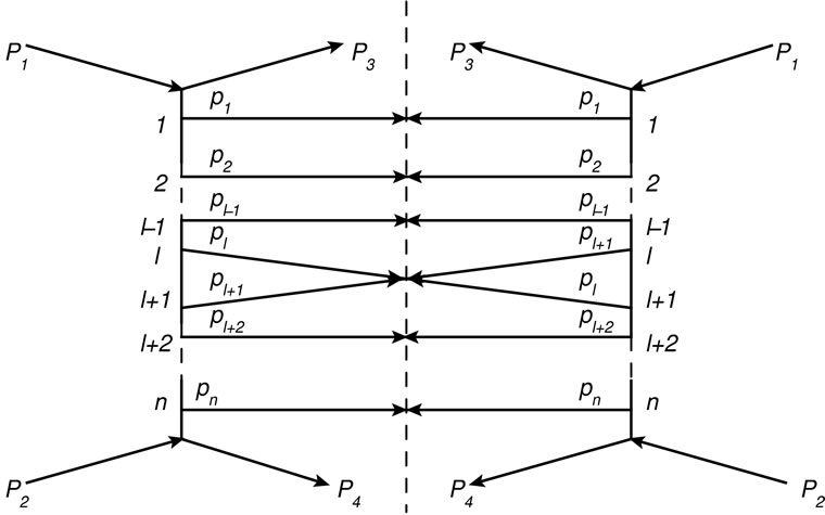
Figure 8. Diagrams, which correspond (n – 1) vectors  closes to vector
 .
.
this case, either a or b would not exceed , i.e., the figure
  contains points, which are at distance less then
  but that cannot happen due to minimality of this distance.
Thus, we can conclude that at an arbitrary n a sphere  can be divided into the parts of equal area, each of which contains only one point of figure
 , as it shown in Figures 7(b), (c).
Let us introduce a multidimensional spherical coordinate system so that the end of vector  is the “north pole” of sphere
 . Then the number of points of figure
  to which the values of variable
  in the interval
  correspond, is equal
 (35)
(35)
where
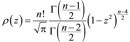 (36)
(36)
 is the Euler gamma function.
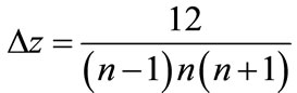
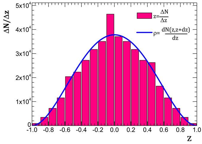
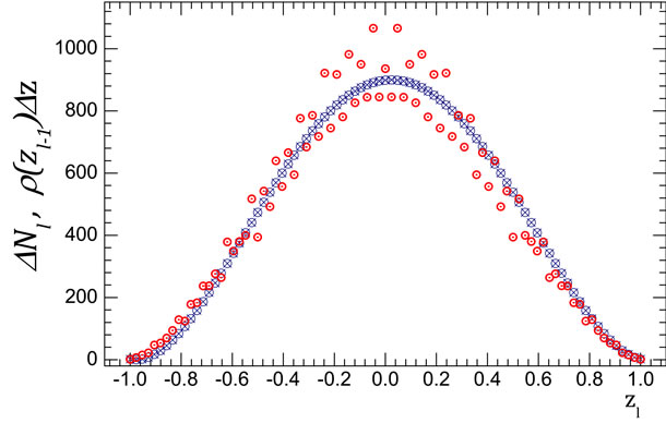
To verify the validity of Equation (35) we can calculate all interference contributions and corresponding values of z at n = 8 and n = 9 (since for the larger number of particles this cannot be realized). The distributions of interference contribution from the variable  and the graphs of function
 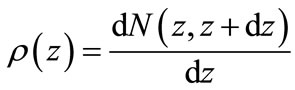 from Equation (35) are shown in Figure 9. Obtained results of numerical calculation of interference contributions and by Equation (35) are in a good agreement.
Moreover, as it follows from Figure 9(b) and from Figure 9(c) this fitness is improved with increasing number of particles n, i.e., Equation (35) is suitable for large n, when the direct numerical calculation of all interference contributions is impossible.
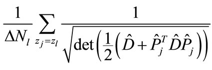
Taking Equation (35) and Equation (9) into account we obtain the following the approximate equality
 (37)
(37)
where
 (38)
(38)
 (a)
(a) (b)
(b)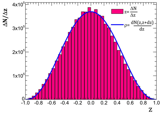 (c)
(c)
Figure 9. Comparison distribution of the interference contribution by the variable  (histogram) and function
  (solid line) at (a) n = 8,
  = 0.1; (b) n = 9,
  = 0.1; (c) n = 9,
  = 0.05. Here
  is the number of interference contributions corresponding to value of
  in the proper interval of
  width.
Verification results of Equation (37) at n = 8 and n = 9 are presented in Figure 10.
Another verification of considered above equations is presented in Figure 11, where the values of  and approximating magnitudes
  (here
(here  is calculated by Equation (29)) are compared.
From results demonstrated on Figure 4 and Figures 10-12, we can conclude that the at least for those numbers of particles for which it can be directly tested Equation (12) with Equation (29), Equations (35)-(37) yields an acceptable approximation. As is obvious from Figure 4, than closer energy to the threshold of n particle production, the better approximation Equation (29). Therefore, if we choose the range of low energies, for example, up to 100 GeV, because in this range total cross-section growth is observed, it is expected that the considered approximations will be acceptable for the large numbers of particles than those for which they were tested. In addition, as it follows from Figures 10(b-d), the accuracy of approximation Equation (37), as expected, increases with the growth of n. Thus, within the framework of examined approximations is possible to calculate the interference contributions at sufficiently large n, and we can consider the dependence of total inelastic cross-section on energy  in the simplest case of multi-peripheral model taking into account all significant interference contributions.
5. The Model of Dependence of Hadron Inelastic Scattering Total Cross-Section on Energy 
Let us consider the magnitude
 (39)
(39)
which within the framework of the discussed above model is an analogue of total inelastic scattering cross-section. Here  is the maximum number of secondary particles allowed by energy-momentum conservation law and
  is the dimensionless coupling constant, which we considered as a fitting parameter (see Equation (32) [2]). Since the calculation of
  up to
up to  takes a long time, so in practice we restrict the upper bound of summation by those values of n, beyond which the neglected contributions known to be smaller than the experimental error of cross-section measurements.
The constant  can be fitted so that the dependence
 looks like the behavior of total hadron-hadron scattering cross-section with a minimum about
  =10 GeV. The result of such a fitting is shown in Figure 13 (in that calculations we take proton mass as mass of primary particles and pion mass as mass of secondary particles).
 (a)
(a)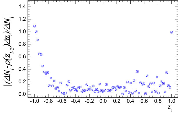 (b)
(b) (c)
(c)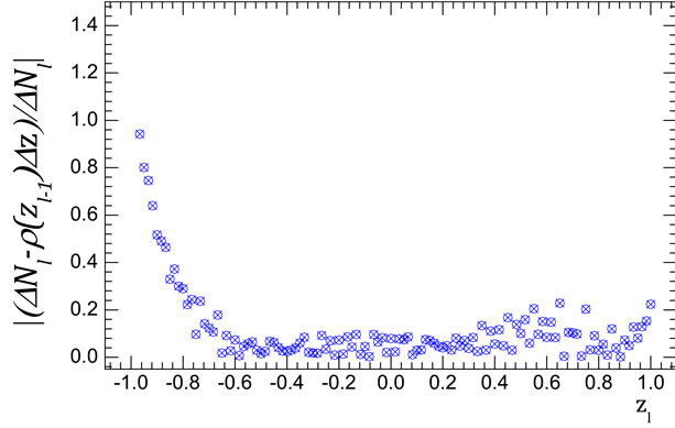 (d)
(d)
Figure 10. Comparison of the values of right-hand side and left-hand side of approximate equality Equation (37) at n = 8 (a, b) and n = 9 (c, d). Circles are the values of  calculated with consideration of for all interference contributions; crosses are the values of function
 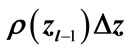 from Equation (35).
 (a)
(a)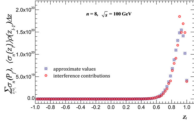 (b)
(b)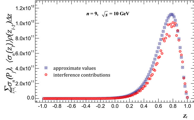 (c)
(c)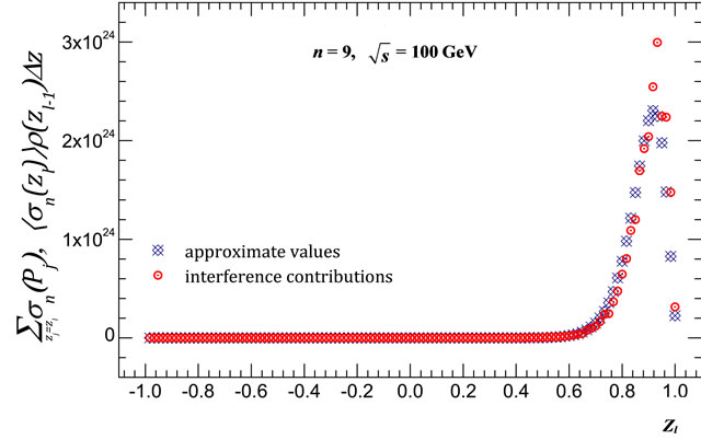 (d)
(d)
Figure 11. Comparison of the values of  obtained with consideration of all interference contributions (circles) and the approximate values of
  (blue crosses) for (a) For n = 8 at
  = 10 GeV; (b) For n = 8 at
 = 100 GeV; (c) For n = 9 at
  = 10 GeV; (d) For n = 9 at
  = 100 GeV.
 (a)
(a) (b)
(b) (c)
(c)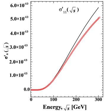 (d)
(d)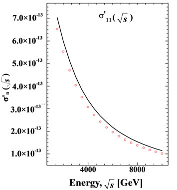 (e)
(e)
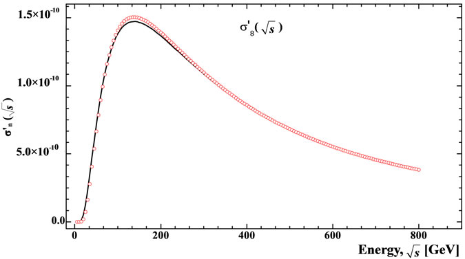
Figure 12. The partial cross-section dependence on energy  calculated over all interference contributions (solid line) and by Equation (12) with the application of approximations Equations (29), (35), (37) (red circles): (a)
 ; (b)
; (b) ; (c)
; (c) ; (d)
; (d) ; (e)
; (e) . This approximation is acceptable at least in the range of parameters in which they are can be verified.
 (a)
(a)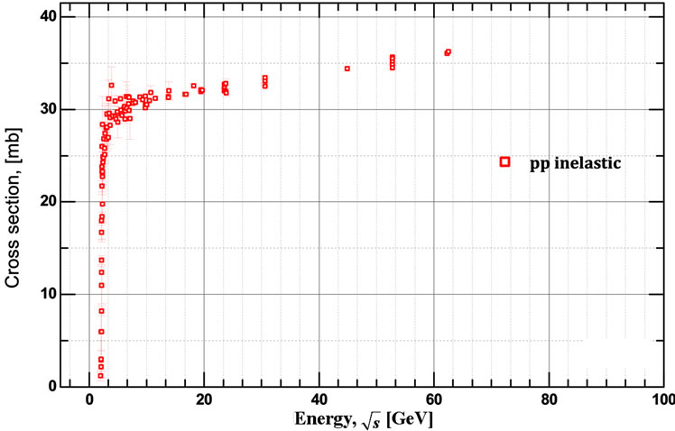 (b)
(b)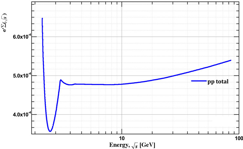 (c)
(c)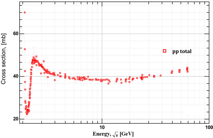 (d)
(d)
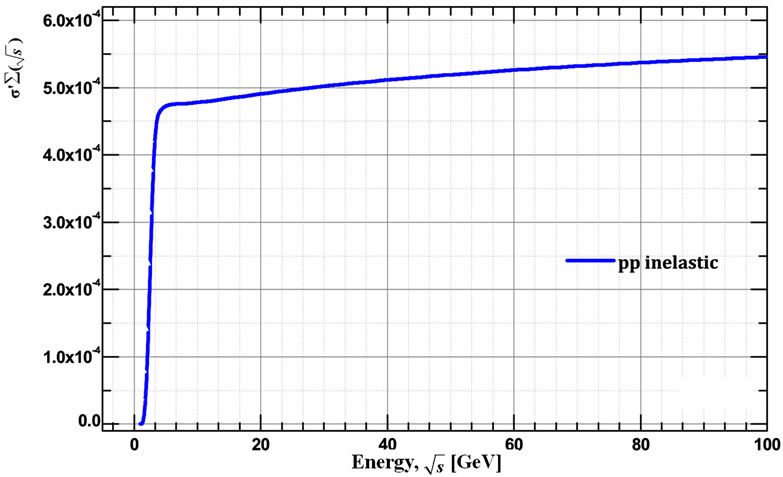
Figure 13. Theoretical dependences of the  (a) and
  (c) obtained for the energy range
  = 1/100 Gev at L = 5.51. First minimum for the total cross-section can be obtained only when we take into account contributions from the high multiplicities. Experimental data for the inelastic (b) and for the total (d) pp scattering cross-section Reference [7,8] presented for qualitative comparison with the prediction from our model. Note: data-points for the inelastic cross-section, obtained from the definition
 .
.
Quantitative comparison with experimental data requires the consideration of more realistic model than the self-interacting scalar  field model.
6. Conclusions
From obtained result, one might conclude that the considered in [1] mechanism of virtuality reduction at the constrained maximum point of multi-peripheral scattering amplitude may be responsible for proton-proton total cross-section growth when all the considerable interference contributions are taken into account.
Just the revelation of mechanism of cross-section growth we consider as the main result of earlier papers [1,2] and present work, since this mechanism is intrinsic not only to the diagrams of the “comb” type, but also to different modifications of considered model.
Application the Laplace method allows to calculate another types of diagrams corresponding to various scenarios of hadron-hadron inelastic scattering and compare it with experimental data.
REFERENCES
- I. Sharf, A. Tykhonov, G. Sokhrannyi, M. Deliyergiyev, N. Podolyan and V. Rusov, “Mechanisms of Proton-Proton Inelastic Cross-Section Growth in Multi-Peripheral Model within the Framework of Perturbation Theory. Part 1,” Journal of Modern Physics, Vol. 2, No. 12, 2011, pp. 1480-1506. arXiv:0605110[hep-ph].
- I. Sharf, A. Tykhonov, G. Sokhrannyi, M. Deliyergiyev, N. Podolyan and V. Rusov, “Mechanisms of Proton-Proton Inelastic Cross-Section Growth in Multi-Peripheral Model within the Framework of Perturbation Theory. Part 2,” Journal of Modern Physics, Vol. 3, No. 1, 2012, pp. 16-27. arXiv:0605110[hep-ph].
- E. A. Kuraev, L. N. Lipatov and V. S. Fadin, “Multi-Reggeon processes in the Yang-Mills theory,” Soviet Physics—JETP, Vol. 44, 1976, pp. 443-450.
- J. Bartels, L. N. Lipatov and A. Sabio Vera, “BFKL Pomeron, Reggeized gluons, and Bern-Dixon-Smirnov amplitudes,” Physical Review D, Vol. 80, No. 4, 2009, Article No. 045002.
- M. G. Kozlov, A. V. Reznichenko and V. S. Fadin, “Quantum Chromodynamics at High Energies,” Vestnik NSU, Vol. 2, No. 4, 2007, pp. 3-31.
- G. S. Danilov and L. N. Lipatov, “BFKL Pomeron in string models,” Nuclear Physics B, Vol. 754, No. 1-2, 2006, pp. 187-232.
- K. Nakamura, “Review of Particle Physics,” Journal of Physics G: Nuclear and Particle Physics, Vol. 37, No. 7A, 2010, Article No. 075021. doi:10.1088/0954-3899/37/7A/075021
- ATLAS Collaboration. “Measurement of the Inelastic Proton-Proton Cross-Section at sqrt{s} = 7 TeV with the ATLAS Detector,” Nature Communications, Vol. 2, 2011, Article No. 463.
NOTES
*Corresponding author.