Applied Mathematics
Vol.5 No.8(2014), Article ID:45235,9 pages DOI:10.4236/am.2014.58103
Positive Periodic Solution for a Two-Species Predator-Prey System
Meiyu Cao, Xiaoping Li*, Xiangjun Dai
Science College, Hunan Agricultural University, Changsha, China
Email: *lxpiii168@aliyun.com
Copyright © 2014 by authors and Scientific Research Publishing Inc.
This work is licensed under the Creative Commons Attribution International License (CC BY).
http://creativecommons.org/licenses/by/4.0/


Received 1 March 2014; revised 1 April 2014; accepted 8 April 2014
ABSTRACT
A two-species predator-prey system with time delay in a two-patch environment is investigated. By using a continuation theorem based on coincidence degree theory, we obtain some sufficient conditions for the existence of periodic solution for the system.
Keywords:Predator-Prey System, Diffusion, Periodic Solution, Coincidence Degree

1. Introduction
Dynamical systems generated by predator-prey models have long been the topic of research interest of many biomathematical scholars, and there have been vast studies to investigate the dynamics of predator-prey models, see e.g., Refs. [1] -[12] and references therein. In 1975, Beddington [13] and DeAngelis [14] proposed the predator-prey system with the Beddington-DeAngelis functional response as follows.
 (1.1)
(1.1)
In the last years, some experts have studied the system [15] -[21] . Recently, Li and Takeuchi [22] proposed the following model with both Beddington-DeAngelis functional response and density dependent predator
 (1.2)
(1.2)
and discussed the dynamic behaviors of the model. In this paper, we consider the following nonautonomous two-species predator-prey system with diffusion and time delays.
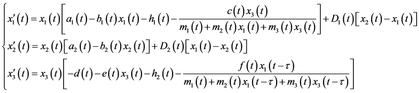 (1.3)
(1.3)
where  represents the prey population in the ith patch
 , and
, and  represents the predator population.
  denotes the dispersal rate of the prey in the ith patch
 . We always make the following fundamental assumptions for system (1.3):
  is positive constant and
 ,
,  ,
,  ,
,  ,
,  ,
,  ,
,  ,
,  ,
,  ,
,  ,
,  re positive continuous
  -periodic functions.
The main purpose of this paper is, by using the coincidence degree theory to derive the sufficient conditions for the existence of periodic solution of (1.3).
2. Preliminaries
The method to be used in this paper involves the applications of the continuation theorem of coincidence degree. we shall use some concepts and results from the book by Gaines and Mawhin [23] .
Let X, Z be real Banach spaces,  be a linear mapping, and
  be a continuous mapping. The mapping L is called a Fredholm mapping of index zero if

and  is closed in Z. If L is a Fredholm mapping of index zero and there exist continuous projectors
  and
and  such that
 ,
,  , then the restriction LP of L to
  is invertible. Denote the inverse of LP by
 . If
. If  is an open bounded subset of X, the mapping N will be called L-compact on
  if
if  is bounded and
  is compact. Since
  is isomorphic to
 , there exists isomorphism
 .
.
Lemma 2.1 (Continuation theorem [23] ) Let  be an open bounded set, L be a Fredholm mapping of index zero and N be L-compact on
 . Assume 1) for each
 ,
, ;
;
2) for each 
3) 
Then  has at least one solution in
 .
.
Throughout this paper, we adopt the notations ,
,  ,
,  where
where  is an
is an  -periodic continuous function.
3. Main Result
Theorem 3.1 Assume that 1) ;
;
2) ;
;
3) ;
;
4) .
.
Then system (1.3) has at least one positive  -periodic solution.
Proof. Let ,
,  ,
,  ,
,  ,
,  then (1.3) can be rewritten as follows:
 (3.1)
(3.1)
where all function are defined as ones in system (1.3). It is easy to know that if (3.1) has one  -periodic solution
 , then
  is a positive
  -periodic solution of system (1.3) Therefore, to complete the proof , it suffices to show that system (3.1) has one
  -periodic solution.
Take  and
and , then X and Z are Banach space with the norm
 .
.
Set ,
,  ,
,  ,
,  ,
, . Obviously,
  ,
,
 is closed in Z and
 . Therefore, L is a Fredholm mapping of index zero. Through an easy computation we find that the inverse
  of
of  has the form
 ,
, . Clearly, QN and
  are continuous. By using Arzela-Ascoli theorem, it is not difficult to prove that
  is compact for any open bounded set
 . Moreover,
  is bounded. Therefore, N is L-compact on
  with any open bounded set
 .
.
Corresponding to the operator equation ,
,  , we have
 . (3.2)
Suppose that  is a solution of (3.2) for an appropriate
 . Integrating (3.2) over the interval
  leads to
 (3.3)
(3.3)
 , (3.4)
 . (3.5)
From (3.2)-(3.5), we have
 (3.6)
(3.6)
 (3.7)
(3.7)
 (3.8)
(3.8)
Multiplying the first equation of (3.2) by  and integrating over
  gives.
 which implies
 (3.9)
(3.9)
By using the inequalities
 .
.
It follows from (3.9) that
 , (3.10)
This yields
 . (3.11)
By using the inequalities
 .
.
It follows from (3.10) that
 . (3.12)
Multiplying the second equation of (3.2) by  and integrating over
 , similarly, we can obtain
 . (3.13)
Substitute (3.13) to (3.12), which leads to

So, there exist a positive constant  such that
 . (3.14)
It follows from (3.13) and (3.14) that there exist a positive constant  such that
 . (3.15)
Substitute (3.14), (3.15) to (3.6) and (3.7), which leads to
 , (3.16)
 . (3.17)
From (3.3) we have
 (3.18)
From (3.4) we have
 . (3.19)
It follows from (3.14), (3.15), (3.18) and (3.19) that there exist  such that
 , (3.20)
 , (3.21)
 . (3.22)
From (3.16), (3.17) and (3.20)-(3.22) we have
 ,
,

 .
.
So, for  we have
 , (3.23)
 . (3.24)
From (3.5) we have

So, there exist  such that
 . (3.25)
From (3.5) we also have
 . (3.26)
It follows from (3.26) that there exist  such that
 .
.
So
 . (3.27)
It follows from (3.8), (3.25) and (3.27) that for  we have
 .
.
So  we have
 .
.
Clearly,  are independent of
 . On other hand, we consider the following algebraic equation
 (3.28)
Take , where
  is large enough such that the solution
  of (3.28) satisfies
 .
.
Let , then
  satisfies the condition (1) in Lemma 2.1. When
 , u is a constant vector in R3 and
 . It follows from the definition of
  that
that , so the condition (2) in Lemma 2.1 is satisfied. In order to verify the condition (3) in Lemma 2.1, we define
  by
by
 where
where  is a parameter. When
 , u is a constant vector in
  and
and . It is easy to obtain that
 , then
 . So,
. So,  is a Homotopy mapping, due to homogoy invariance theorem of topology degree, we have

It is not difficult to see that the following algebraic equation

has a unique solution

Thus

By now we have proved the condition (3) in Lemma 2.1. This completes the proof of Theorem 3.1.
References
- Freedman, H.I. (1980) Mathematical Models in Population Ecology. Marcel Dekker, New York.
- Sugie, J. (1998) Two-Parameter Bifurcation System of Ivlev Type. Journal of Mathematical Analysis and Applications, 217, 349-371. http://dx.doi.org/10.1006/jmaa.1997.5700
- Ardito, A. and Ricciardi, P. (1995) Lyapunov Functions for a Generalized Gause-Type Model. Journal of Mathematical Biology, 33, 816-828. http://dx.doi.org/10.1007/BF00187283
- Hassel, M.P. (1978) The Dynamics of Arthropod Predator-Prey Systems. Princeton University Press, Princeton.
- Hwang, T.W. (1999) Predator-Prey System. Journal of Mathematical Analysis and Applications, 238, 179-195. http://dx.doi.org/10.1006/jmaa.1999.6520
- Hsu, S.B., Hwang, T.W. and Kuang, Y. (2001) Global Analysis of the Michaelis-Menten Type Ratio-Dependent Predator-Prey. Journal of Mathematical Biology, 42, 489-506. http://dx.doi.org/10.1007/s002850100079
- Kot, M. (2001) Elements of Mathematical Biology. Cambridge University Press, Cambridge.
- Kuang, Y. and Freedman, H.I. (1988) Uniqueness of Limit Cycles in Gause-Type Predator-Prey Systems. Mathematical Biosciences, 88, 67-84. http://dx.doi.org/10.1016/0025-5564(88)90049-1
- Kooij, R.E. and Zegeling, A. (1996) A Predator-Prey Model with Ivlev’s Functional Response. Journal of Mathematical Analysis and Applications, 198, 473-489. http://dx.doi.org/10.1006/jmaa.1996.0093
- Liu, X.X. and Lou, Y.J. (2010) Global Dynamics of a Predator-Prey Model. Journal of Mathematical Analysis and Applications, 371, 323-340. http://dx.doi.org/10.1016/j.jmaa.2010.05.037
- Xiao, D.M., Li, W.X. and Han, M.A. (2006) Dynamics in Ratio-Dependent Predator-Prey Model with Predator Harvesting. Journal of Mathematical Analysis and Applications, 324, 14-29. http://dx.doi.org/10.1016/j.jmaa.2005.11.048
- Xiao, D. and Zhang, Z.D. (2003) On the Uniqueness and Nonexistence of Limit Cycles for Predator-Prey Systems. Nonlinearity, 16, 1185-1201. http://dx.doi.org/10.1088/0951-7715/16/3/321
- Beddington, J.R. (1975) Mutual Interference between Parasites or Predators and Its Effect on Searching Efficiency. Journal of Animal Ecology, 3, 331-340. http://dx.doi.org/10.2307/3866
- DeAngelis, D.L., Goldstein, R.A. and O’Neil, R.V. (1975) A Model for Trophic Interaction. Ecology, 4, 881-892. http://dx.doi.org/10.2307/1936298
- Cantrell, R.S. and Cosner, C. (2001) On the Dynamics of Predator-Prey Models with the Beddington-DeAngelis Functional Response. Journal of Mathematical Analysis and Applications, 257, 206-222. http://dx.doi.org/10.1006/jmaa.2000.7343
- Chen, F., Chen, Y. and Shi, J. (2008) Stability of the Boundary Solution of a Nonautonomous Predator-Prey System with the Beddington-DeAngelis Functional Response. Journal of Mathematical Analysis and Applications, 344, 1057- 1067. http://dx.doi.org/10.1016/j.jmaa.2008.03.050
- Cui, J. and Takeuchi, Y. (2006) Permanence, Extinction and Periodic Solution of Predator-Prey System with the Beddington-DeAngelis Functional Response. Journal of Mathematical Analysis and Applications, 317, 464-474. http://dx.doi.org/10.1016/j.jmaa.2005.10.011
- Dimitrov, D.T. and Kojouharov, H.V. (2005) Complete Mathematical Analysis of Predator-Prey System with Linear Prey Growth and Beddington-DeAngelis Functional Response. Applied Mathematics and Computation, 162, 523-538. http://dx.doi.org/10.1016/j.amc.2003.12.106
- Fan, M. and Kuang, Y. (2004) Dynamics of a Nonautonomous Predator-Prey System with the Beddington-DeAngelis Functional Response. Journal of Mathematical Analysis and Applications, 295, 15-39. http://dx.doi.org/10.1016/j.jmaa.2004.02.038
- Hwang, T.W. (2003) Global Analysis of the Predator-Prey System with the Beddington-DeAngelis Functional Response. Journal of Mathematical Analysis and Applications, 281, 395-401. http://dx.doi.org/10.1016/S0022-247X(02)00395-5
- Liu, S. and Beretta, E. (2006) A Stage-Structured Predator-Prey Model of Beddington-DeAngelis Type. SIAM Journal on Applied Mathematics, 66, 1101-1129. http://dx.doi.org/10.1137/050630003
- Li, H.Y. and Takeuchi, Y. (2011) Dynamics of the Density Dependent Predator-Prey System with Beddington-DeAngelis Functional Response. Journal of Mathematical Analysis and Applications, 374, 644-654. http://dx.doi.org/10.1016/j.jmaa.2010.08.029
NOTES

*Corresponding author.