ABSTRACT

This paper introduces the optimal foreign exchange risk hedging model following a standard portfolio theory. The results indicate that a lower level of risk can be achieved, given a specified level of expected return, from using optimization modeling. In the paper the expected hedging return is defined from the expected cost of the foreign currency using a specified hedging strategy minus the expected cost of the foreign currency when it is purchased form the spot market. The focal point of the technique is its ability to identify optimal combinations of hedging vehicles, those are currency options, forward contracts, leaving the position open (foreign exchange risk hedging tools suggested by the US. Department of Commerce) in a closed form.

1. Introduction

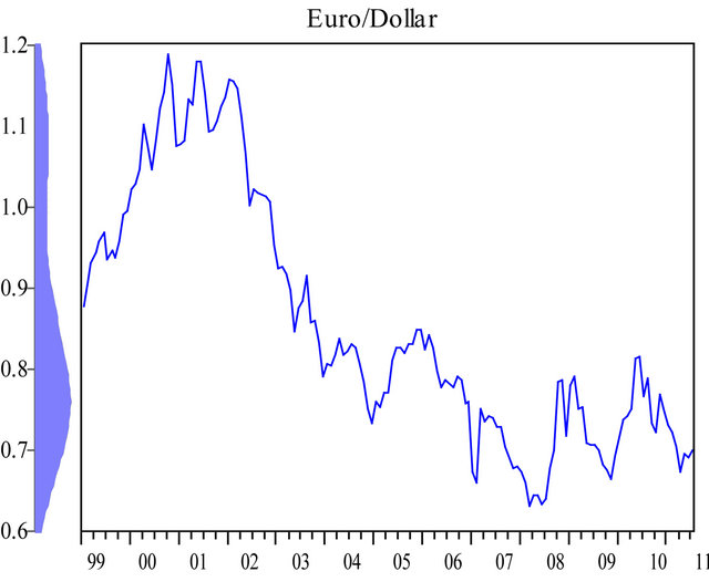
Beginning in the early 1970s, floating foreign exchange (FX) rates became more common, among the major currencies. Now the recent global financial crisis including euro zone instability have clearly illustrated the critical importance of hedging for risks in foreign exchange rate. See following figures of monthly Euro/Dollar and Yen/ Dollar foreign exchange rates during 1999.1-2011.7, where both FX rates are fluctuating especially after global financial crisis.¹

So foreign currency fluctuations are one of the key sources of risk in multinational operations. The various tools which have emerged to deal with foreign exchange risk have been treated extensively in the finance literature. The nature, uses, and efficiency of their markets are quite well understood today (See [1]). The US Department of Commerce is also warning that “The volatile nature of the FX market poses a great risk of sudden and drastic FX rate movements, which may cause significantly damaging financial losses from otherwise profitable export sales (Trade finance guide, http://trade.gov /publications/pdfs/tfg2008ch12.pdf).” The same guide suggests three FX risk management techniques considered suitable for new-to-export US small and mediumsized enterprises companies as non-hedging FX risk management techniques,² FX forward hedges³ and FX options hedges.⁴

However, what has been ignored, as correctly pointed out [2], are the factors an investor should consider when choosing from among the various available hedging tools to reduce the risk resulting from a certain type of exposure to foreign exchange risk for a given expected return.

[2] gauges the preferences of finance officers in terms of the specific characteristics of a hedging tool relying on a questionnaire survey. [3,4] illustrate the technique of computerized optimization and simulation modeling to manage foreign exchange risk. However they did not derive the closed form optimal hedging solution analytically and thus it obviously requires the additional computational burden.

So this paper introduces the optimal foreign exchange risk hedging model following a standard portfolio theory. The results indicate that a lower level of risk can be achieved, given a specified level of expected return, from using optimization modeling. In the context of this paper the expected hedging return is defined from the expected cost of the foreign currency using a specified hedging strategy minus the expected cost of the foreign currency when it is purchased form the spot market. The focal point of the technique is its ability to identify optimal combinations of most frequently using hedging vehicles, those are (European) currency options, forward contracts, leaving the position open (foreign exchange risk hedging tools suggested by the US Department of Commerce) in a closed form.⁵

The rest of this paper proceeds as follows. Section 2 derives the expected return and variance of hedging vehicles. Section 3 analyzes the optimal hedging selection. Section 4 concludes.

2. Moments of Triple Hedging Tools’ Returns

Assume, at time 0, an investor hopes to buy one unit of foreign exchange at a future time. Denotes as the foreign exchange rate at time in terms of domestic currency. For instance, is the dollar price of one euro where the dollar is the domestic currency. Further we suppose that there are three hedging tools, i.e., European currency call option, forward contracts and leaving the position open.⁶ Define a forward contract rate, a striking price and its premium at time t of European call option with the maturity, respectively.⁷

Now we would like to construct the efficient hedging frontier composed of expected return and variance of each hedging vehicle. So, it is exactly matched with the portfolio possibilities curve. An optimal combination of hedging vehicles is one, which maximizes the expected return given a desired level of risk.

Before proceeding, we assume the logarithm of exchange rate follows a random walk following [5]:

Assumption 2.1. We suppose

where and is independent, identically and normally distributed sequence with the mean zero and variance.

Above Assumption 2.1 represents the efficient market hypothesis for the foreign exchange rate. Now we derive the return and its variance of different hedging tools, where the return is computed based upon the purchasing a foreign currency by the spot rate. The expected return is defined from the conditional expectation⁸ based on the information of past exchange rates .⁹

2.1. Derivation of Mean and Variance

At first, we derive the expected return [R_n] and its variance [V_n] of non-hedging (leaving the position open) as:

Proposition 2.2. Suppose Assumption 2.1 holds. Then the expected return for non-hedging is and its variance is.

Proof. Note the return of non-hedging is the negative¹⁰ value of following:¹¹

(1)

assuming is small. Then, under Assumption 2.1, the claimed results hold as:

and

.

At second, we derive the expected return and its variance of forward contract as:

Proposition 2.3. Suppose Assumption 2.1 holds. Then the expected return of forward is and its variance is where.

Proof: Note the expected return for forward is the negative value of following:

assuming is small. Its variance is obviously zero since the return is not random.

Above forward contract may dominate the non-hedging if its expected return is positive, which is riskless. Such dominance may be closely related with the interest rates whenever the covered interest parity holds. See following result.

Corollary 2.4. Suppose Assumption 2.1 holds and. Then the forward contracts dominates the nonhedging where and denote the domestic and foreign risk free interest rates respectively.

Proof. From the covered interest parity, note =. So if or, then there is positive expected return without risk. In this case, the forward contract dominates the non-hedging case.

Above result also implies that if the domestic interest rate is higher than the foreign interest rate, then the non-hedging may better than the forward contract.¹²

Now we derive the expected return [R₀] and its variance [V₀] of currency call option as:

Proposition 2.5. Suppose Assumption 2.1 holds. Then 1) the expected return of currency call option is given as:

and 2) its variance is

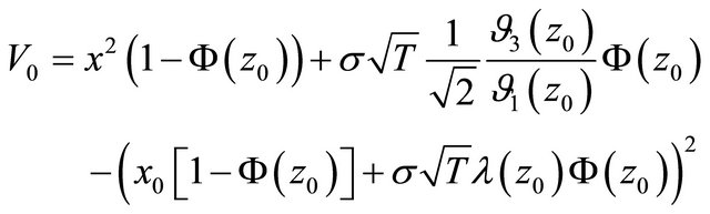
where, , ,

and where and are the standard normal density and distribution function respectively and denotes the distribution function of distribution with the degree of freedom.

Proof. 1) Note the outflow of call option at time is given as where is the option premium. Thus its return is the negative value of following:

assuming and are small.

Now the expected return conditional on is the negative value of following:

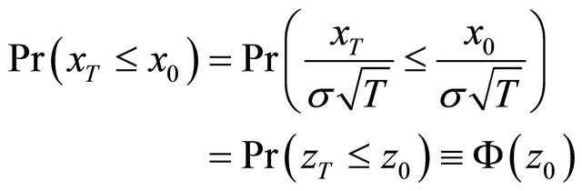
where, since

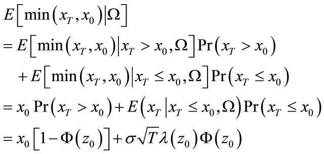(2)

from the definition of conditional expectation, where from Assumption 2.1 and

(3)

for the Equality (2) from [7] (p. 759), and

where.

2) The return’s variance of call option conditional on is defined as:

(4)

Note the second term of (4) is derived from (2) directly. Then the first term of (4) is arranged as:

(5)

from the definition of conditional expectation for the first equality.

However we may show

(6)

from following facts (b-i) and (b-ii):

(b-i)

since 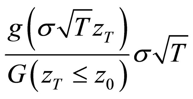is the truncated density function of variable since

from the change of variable formula where and denote the density and distribution functions of respectively, and since by definition.

(b-ii)

from [8] (Remark 3), where

andwhere

and

in [8] (Remark 3) where.

Finally if we plug (6) into (5), then we get the claimed result as:

2.2. Derivation of Covariances

At second, we derive the covariance among three hedging tools. Note the covariance of returns between nonhedging (or option) and forward is obviously zero since the forward return is not random. Then the covariance of returns between option and non-hedging is given as:

Proposition 2.7. Suppose Assumption 2.1 holds. Then the covariance of returns between option and non-hedging is

Proof. Note the covariance between non-hedging and option conditional on is defined as:

since the fourth equality holds from

Now the claimed result is derived since

from (3) and (6) for the last equation and

.

3. Efficient Hedging Frontier Construction

Based upon above derivation of return structure, now we may derive the efficient hedging frontier. It is exactly matched with the portfolio possibilities curve in a standard portfolio theory (see [9] for a nice introduction).

For this purpose, first of all, we consider a portfolio composed of non-hedging and call option that are all risky. Let the weight of non-hedging be as w and 1 − w for the option where w is a number. Then, from the above derivation, its expected return is defined as:

and its variance is given as:

where denotes a covariance between the returns of non-hedging and call option.

In our case, the return of forward has the zero variance with the expected return is. Thus it is regarded as the riskless asset in the standard portfolio theory. Now the hedging allocation line¹³ connecting the riskless forward contract and a combination of non-hedging and call option is defined as:

(7)

where denotes the return and denotes the risk;

is a slope.

Then the efficient hedging allocation line¹⁴ is given by solving following problem:

(8)

that is maximizing the slope of Equation (7) with the argument w.

The problem (8) may be solved without restriction by [9] (pp. 100-103) as:

(9)

where

.

If or, then the maximization problem (8) should be solved under the restriction using a typical Kuhn-Tucker condition.

Finally, the efficient hedging frontier is given by

(10)

where.

For the given efficient frontier in (10), optimal hedging (c.f., separation theorem) is conducted as follows. At first, the hedging ratio between non-hedging and option re set as. At second, is set for the forward and is set for the first combination of non-hedging and option. Expected utility maximization may be a rule to determine a. Finally

becomes the optimal hedging ratio of the forward, non-hedging and call option. See following Figure 1.

Now we suggest an example that shows how above result may be applied in the field.

Example 3.1. Above result is applied to the dollar as domestic currency and the yen as the foreign currency. To compute the efficient hedging frontier in (10), we let months, (August 18, 2010),

, , dollar/100yen and an estimator of (during 2005.1- 2009.12).

Then, at first, we get, , , , and from the above results. Then we obtain the return

and variance of the portfolio non-hedging and option where.

From this result, the Equation (10) in the efficient hedging frontier becomes:

₍₁₁₎

Suppose an extremely risk-averse investor maximizes

a utility function subject to (11).¹⁵ The resultant portfolio induces and. It implies where the utility is maximized with the constraint (11). Thus the forward, non-hedging and option are finally selected as

4. Conclusion

We introduced the optimal foreign exchange risk hedging model following a standard portfolio theory. The results indicate that a lower level of risk can be achieved, given a specified level of expected return, from using optimization modeling. The structure may be extended to cover the futures and American options and we will take it as a future research topic. However I am sure the similar logic may be readily applied to these extensions. Further a development of convenient computer program for FX risk hedging users based on above results might be a useful project.

REFERENCES

NOTES

¹The axsis border graphs are kernel density functions.

²The exporter can avoid FX exposure by using the simplest non-edging technique: price the sale in a foreign currency. The exporter can then demand cash in advance, and the current spot market rate will deterne the US dollar value of the foreign proceeds.

³The most direct method of hedging FX risk is a forward contract, which enables the exporter to sell a set amount of foreign currency at a pre-agreed exchange rate with a delivery date from three days to one year into the future.

⁴Under an FX option, the exporter or the option holder acquires the right, but not the obligation, to deliver an agreed amount of foreign currency to the lender in exchange for dollars at a specified rate on or before the expiration date of the option. As opposed to a forward contract, an FX option has an explicit fee, which is similar to a premium paid for an insurance policy.

⁵At least author’s knowledge, there are not any the same researches in this direction.

⁶It is a non-hedging and to buy the foreign currency at time.

⁷The value of call option was derived by [6].

⁸Note the conditional expectation is the optimal forecasting of return which minimizes the mean squared forecasting error.

⁹So an investor exploits the information when she determines the optimal hedging tool.

¹⁰It is negative because buying of foreign currency means the outflow of domestic currency.

¹¹We do not consider the cost-of-carry for the spot purchasing of foreign currency since it is applied for the other hedging vehicles by the same amount. In particular, suppose an interest is required to borrow the till time and then the non-hedging return Formula (1) may be revised as;

Thus it does not matter even if we just focus on the since the other terms and are same for the other hedging tools.

¹²This result well explain why a lot of firms of the developing countries with the high interest rate do not use the forward contract. The problem is the cost to use the forward is bigger than the non-hedging if even though there is the risk difference.

¹³It is called as the capital allocation line in the portfolio theory.

¹⁴It is called as the capital market line in the portfolio theory.

¹⁵This utility function largely penalizes the risk and reflects deep risk aversions (e.g., under recent financial crisis). Of course other utility functions may be readily applied.