Open Journal of Geology
Vol.06 No.11(2016), Article ID:71755,19 pages
10.4236/ojg.2016.611098
Sarvak Formation Reservoir Modeling, in Oilfield Kuhmond (Southwestern Iran)
Jafar Qomi Aveili*
Islamic Azad University of Chalus, Chalus, Iran

Copyright © 2016 by author and Scientific Research Publishing Inc.
This work is licensed under the Creative Commons Attribution International License (CC BY 4.0).
http://creativecommons.org/licenses/by/4.0/


Received: July 4, 2016; Accepted: October 31, 2016; Published: November 3, 2016
ABSTRACT
Sarvak formation is one of the important hydrocarbon reservoirs in the Zagros Basin that is one of the mid-Cretaceous carbonate units in Bangestan. This formation is located in the Kazhdomi Formation with the same slope. Geology, Kohmond field is located in the southeast of Bushehr and north and northwest of the Fars province. In this project, the geology, the tank and Petrophysics features were studied in the field with sedimentology; stratigraphy, Petrophysics, sedimentary environments and reservoir data analysis. According to studies, sedimentary environment of Sarvak in the Kohmond field is diagnosed as a ramp carbonate platform. Sarvak reservoir modeling in this field was done by using Petrelli software. The results indicate parts with high porosity, which are focused more in central and southeastern parts of the field and can contain large amounts of oil.
Keywords:
Sarvak Formation Reservoir Modeling, Oilfield Kuhmond

1. Introduction
One of the most important petroleum basins in the Middle East is Zagros Basin that the largest of the Iran reservoirs is located in the geological zone of the Zagros and Basin in the Persian Gulf (1980 murris). In this study, the evidences were obtained based on heavy oil in Asmari Jahrum formation and Bangestan group “Kohmond”. And because the depth of these formations was low in the Monde field 250 - 1500 m and the reservoir has also been considerable dimensions (12.5 × 72.5 km), the reservoir of Sarvak in this field is considered as the first heavy oil exploration field.
Sarvak formation is a thick carbonate stratigraphic unit that is part of Bangestan group; it is deposited in the Zagros region, and the southern fringe of Neotitis. According to James and Wynd’s report in 1965 from the Albian to Campanian, a sedimentary cycle of Kazhdumi formations, Sorga, Ilam, Sarvak can be identified in the Zagros that set list is called the Bangestan group. Jahrum and Sarvak formations are two heavy oil reservoirs in the oilfield of Kohmond (Figure 1).
2. Method
By using Petrol software and petrophysical charts, we have built a static and functional geological model. Naming carbonate facies were done based on the category of full and Dunham [1] , but due to the importance of naming Dunham in the oil industry, the Dunham classification method was used in this study.
2.1. Geographical location
Kohmond square is a heavy oil field that is the largest heavy oil fields in southwestern

Figure 1. Kohmond on the gulf coastal side, satellite photos (Google earth).
of Iran. This field is located in 70 kilometers of southeast of Bushehr on the Persian Gulf and in plain areas. Kohmond field has a length of about 90 km and a width of 16 km. In addition, it has the direction of North West and the South East and has been drawn in the form of an anticline structure.
2.2. History of Drilling
For the first time, reserves of Kohmond were discovered in 1931 and many excavation were done on it [2] , so that, in the years (1931 to 1932), Monda well was excavated in the method of rotating drilling and impulsive alternatively, in order to assess Bangestan tanks and Asmari, to a depth of 1169 meters (Sarvak) [3] .
Monde Wells 2 to 5 were excavated between 1960 and 1976. The purpose of drilling these wells was reaching to the group “Dah Ram” and assessing of gas in these tanks. No. 6 was excavated in 1984, to evaluate the too heavy oil tanks of Jahrum, Ilam, Sarvak and Asmar and finally, wells No. 7 was excavated in 1986, to evaluate and obtain more complete information from the field and achieve very heavy oil of Jahrum and Sarvak. In 2005 to 2006, excavating operations of well No. 8 was performed. In this field, 8 wells have been excavated till now, that the deepest of them is wells (5) with the action of 5055 meters.
Generally, in this field, the number of wells in a straight line is excavated that are almost in line with the South East to the North West along the anticline. According to the figure below, it can be explained that, most of these wells are located in the center of the anticline (Figure 2).

Figure 2. View of the drilled wells’ location in the Kohmond area, Sarvak page (software petrel 2009).
2.3. Sarvak Formation Stratigraphic Situation in Kohmond
The age of the formation in the area is considered Upper Cretaceous based on studies conducted (Turonian-Cenomanian) [4] . The sediments of this formation are gray lime- stones that are pure in areas containing pyrite, oolite and sometimes lime. The middle and lower part of the formation are formed of the gray and dark brown layers of marl with inlayer cream-colored and occasionally Chile and in some areas slumberous calcareous rocks [5] .
According to studies, Sarvak formation has two zones in the study area. These zones include Ahmadi or “shale Ahmadi” and Madood or Medved part that are known as “lime Medved”.
Ahmadi section: from gray to green shale with thin bedded limestone.
Medved section: from gray to green shale with thin bedded limestone. This part is more pure lime. The bottom line of this Formation with Kazhdumi formation is almost gradual and there is no unconformity.
Fossils of this formation are:
Gastropoda sp. or biTolina concave. Trochlina spp Shell fragm. sp.
According to studies conducted in Sarvak formation in the Kohmond field, Oligostegina fossils have the most frequency among other things. The following fossils have been observing a lot in this formation.
Globigerina. sp, Echinoderm. sp. Rudist. sp.-pelecypod.
2.4. Structural Geology of the Zone
The Zagros Fold along with part of Azerbaijan that sediments happen during the Silurian to the Permian, probably formed part of the platform in the Iran Paleozoic. Eftekhar Nejad, 1980, it looks like the Zagros was the vibrant and marginal part of Arabic page and during the late phase of sedimentation in this area, the steeped land in effect, of gradual change along the compression forces, axis of folds is oriented to the South West. In connection with the study area, as shown in Figure 3, the right-turn movement of fault that is known as the Qatar-Kazeroon fault, has created changes in the northern part of the stalactites Kohmond (nose), so that it has twisted the nose of the Koohmond anticline to the north [6] . It has increased significantly and oriented the fractures in the studied buildings.
Kohmond is a symmetrical anticline with 16 km wide and 90 km long on the coast of the Persian Gulf and South East of Bushehr. Its vertical dependency on Ilam formation is about 6300 meters and on Jahrom, formation is 3500 meters. Aghajari, Bakhtiari, Mishan, Gachsaran formations formed the protrusions on the field. Mishan and Aghajari and Bakhtiari formations, respectively, are placed to the edge of the field and Gach- saran formation were scattered in the middle hump [7] .
A southwestern ridge of anticline Kohmond in southern Bushehr-Delaware Birikan, the photo represents the erosion in Aghajari formation located in the southwestern ridge of anticline. Also an angluar discontinuity between Aghajari and Bakhtiari formations re- present an orogenic phase in the region. Look is toward the East. Adapted from [8] .

Figure 3. The impact of Kazeroon-Qatar right-turn fault in Koohmond anticline of vector red is the color of northerly direction indicator. (google earth).
On the surface, anticline axis has been moved by numerous faults near and in the middle of the plunge.
Results of sections that have been ticked in this area indicate that, Kohmond is a very simple anticline and its edges are extended with relatively gentle slope and perfectly symmetrical. The average slope of this anticline, on its southern slope is 15˚ and on the northern slopes is 17 degrees. In general, the kind of fold in this field is consistent with the overall trend of folding in southern Iran. Even we can say that the movements of Hormuz Salt have been effective in its formation [9] .
2.5. Reservoir Modeling
The two-dimensional modeling technique was used during many years in reservoir characterization as a primary method. Increasing our knowledge, and improving the quality of reservoir data, gives us the conclusion that the above methods are insufficient. In addition, reservoir simulation has been done for a long time, based on a three- dimensional classification. Therefore, a three-dimensional model depending on reservoir engineers and geologists in a comprehensive study of a reservoir are very important [10] .
Reservoir modeling is the main core of reservoir studies that, with reservoir simulation software, it is created from a combination and modeling with a series of dynamic and static parameters. One of the largest matters that make the modeling hard is the lack of information. As a result, at best, a few models are created for the reservoir, which have differences. However, in this study, by using the following methods, it has been tried to reduce the modeling error to a minimum.
(Neural network, Kriging, Sequential Gaussian simulation).
Several factors are making the reservoir modeling process more complex, including the following:
1) The presence or role of fractures.
2) The multistage diagenetic history that creates a range of pore complex network in Microborta Megacarset scale [11] .
3) The structure of heterogeneous stratum.
2.6. Needed Information
A lot of information is required for each modeling, that if the information will be more accurate and perfect, the model is closer to the real tank and is more resemble and could have many applications. It should be noted that, due to high costs, and despite the difficulties and obstacles that make the logging and wells logging hard, in most cases, not all the required information in full can be possessed and this is the art of model- makers to use the information and statics they have and present the best reservoir model that represents the real environment and reservoir features. These information include: geometry, coordinate of the wells, petrophysical logs (including diagrams of Sonic, gamma, neutron, resistivity, porosity, density, circuit diagrams, etc.), or Facieslog, Information of fractures, permeability or porosity, Sizomic information, building plans or UGC, outlines of formations, the final report of shafts, petrophysical reports.
2.7. Modeling Software
By using three-dimensional drawings and software of the reservoir in the computer, diagnosis unbiased tank units will be much easier. It also uses the model created, and the porous units in different parts of the tank, especially away from the main part of the tank can be revealed that, without the use of software and having a three-dimensional view of the area, it would easily not available. By using three-dimensional modeling, a lot of trials and errors answers and data required for reservoir can be obtained without the need for conventional drilling, which these information reduces the cost of extracting and faster access to energy resources.
2.8. Petrel Software
Due to mature fields reservoirs management, a modeling tool requires that stimulates the wells quickly and gives the shape of the geological models of one-dimensional, two-dimensional and three-dimensional to the model-makers, so that they could manage all existing oil wells in the region, and to that end, for the first time, the software Petrelli was designed by Schlumberger.
Petrelli has created the capability for the user to interpret the seismic data, perform matching between different wells (Well correlation), make a suitable model for reservoir simulation, present the results and charts for simulation reports, draw maps, calculate the volume and present development plans and strategies that lead to maximum utilization from storage. This research is used Sarvak modeling from Petrelli software [12] .
2.9. The Input Data (Input Data)
The first step in entering the well head modeling or information about the coordinates of the wells, their lineup, the distance from the Earth’s surface to drilling rotary table (KB), the point of entry to the reservoir wells (Top Depth) and end point of drilling of each well in a tank (Bottom Depth) and also the Symbol of per well. This information can be in prepared way and in a file or can be made by using the drilling reports in a file by Excel software. Then, after the cell is classified, it enters into the application Petrelli as a text file [13] .
Second stage is related to data entry Well Top, that at this stage, we enter information related to the formation (Top Formation). At this stage, as before, in the absence of Digital files or the same method, we make these files and enter the related information as a text file into our application [14] .
In the next step, we enter the well Log information or petrophysical logs, which are digitized into their own wells. These charts include charts of neutrons, permeability, resistivity, gamma, etc. By using the well Section window, we can analyze petrophysical logs (blogs) clearly and precisely, even with the use of interpretations of figures such as gamma. It is possible to identify new zones or changes in the existing zones. The different wells can be put together to match (Correlation) and in different depths and layers, their lithology characteristics are examined [15] (Figure 4).
2.10. Creating Facies Charts (Facieslog)
By using template Windows, facies in their own wells can be created and specified it in different parts of the wells. That is, at first, a certain color and shape (Style) will be chosen for each type of facies as a model, and then a different depth should be in the desired color and shape. For example, create a facies pattern in which the yellow color and brick form should be ascribed to a dense limestone. Then, after interpreting logs,

Figure 4. Show zoning of Sarvak formation by using gamma log in the field, also facies chart is specified on the left side (well section).
we conclude that, from a depth of 1150 to 1153 m, corresponding to the dense limestone. By using a set pattern, we paint the desired depth. After determining the pattern, for different parts of the formation and painting all parts of it, we have a facies chart, that by seeing the yellow color with the brick form, at different depths from each of the wells, we conclude that, there is a dense limestone in that part.
In addition, you can operate the automatic painting and by software, which is created by using the formula in the calculator, the action is possible.
For example, when the gamma curve becomes greater than 40%, we want all parts of the wells will be yellow line, and with applying the formula in the Calculater, this action will be performed. It should be noted to perform this function; you first need to have studies done on the well logs, to choose the best method and formula, and then by using this information, select the best method, and proceeded to build the chart facies.
2.11. Thickness Map
The thickness of the layers can be calculated in several different ways, and each one obeys its own rules. One of these methods is using spreadsheets menu, which by using this field, and subtracting various acts from high points; we obtain the thickness in different parts of our wells. It should be kept in mind that, this is hard, tedious and time-consu- ming, and we must seek another way than this, because in reservoirs that the number of wells is more than a few dozen, doing this to get the thickness of the layer is very time consuming and error. To simplify this task, by using the practice of making thickness maps or ISO point, from two considered layers (the layer that we want to obtain the thickness between them), we create a thick page, on this page, information on different parts of the formation is visible for the user and the thickness of each point can be examined alone (Figure 5).
2.12. Modeling
In Petrelli, three-dimensional modeling, it can be divided into three stages that each of which is dependent on others, these steps include:
1) The property modeling
Structural modeling is stratigraphic modeling.
2) The stratigraphic modeling
In the stratigraphic modeling, reservoir formations and the available zones are designed, the created models, according to space parameters x, y, z was three-dimensional and for modeling, petrophysical and dynamic properties and various analyzes will be available in other parts of the software [13] [14] [15] (Figure 6).
3. Reservoir Structural Modeling
Structural modeling is a griding reservoir and the construction of reservoir framework, so that all data, statistics, and construction information can be observed as a three-dim-

Figure 5. View the surface with the same thickness as Sarvak layer in oil field of Kohmond; see from east side of field (petrel 2009).
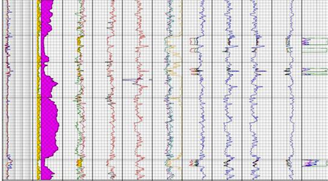
Figure 6. View of petrophysical charts from wells in Kohmond (gamma charts with green color, notron with blue color and porosity is specified with red color).
ensional model. Our information and data are always limited relative to the size, complexity and size of the reservoirs. By using the structural modeling, the reservoir can be divided as the same mesh network that all the properties of each cell of this network such as lithology petrophysical properties at all levels are almost identical. In addition, Due to the network distance from each other, and the information and statistics for each of them, we can estimate different properties in cells that lacked any information. The more knowledge of the grid cells, we have, the estimate will be closer to reality. In the structural modeling, various stages will be done, respectively, include the following [16] :
1) Fault modeling
2) Pillar gridding
3) Make/Edit horizons
4) Make/Edit zone
5) Layering
A) Fault modeling
At this point, we have to enter the information that is relevant to the fault, to the software, if, as in this study, there were no information and statistics available from regional fault, by using the additional information and reports and from the pages, they are recognized, by using the pillar gridding, we proceeded to build them manually. In addition, it should be noted that, to do this, you must use a two-dimensional plane.
Fault modeling with the use of Structural modeling begins after drawing the fault line. To do this, at first we focus on a three-dimensional plane that whether the fault line created on the surface agrees or not. If the fault line was not on the surface and it was in the space above or below the surface, with using the calculation, we make the coordinates of the surface and the fault line the same so that the fractures created will be matched on the surface. Therefore, with the use of fault modeling, we proceeded to build the model of these faults. We choose the option for making fault on the polygon and divide the fault line to three-dimensional pillars. After doing this, we limit all faults (fault) by using the limited options between surfaces so that during the modeling, the lines will not be removed from the formation surface. Therefore, we connect the faults that have collided together. This connection must be done in such a way that the relationship between these lines together will be without any interval. In the meantime, they do not interfere with each other [16] . At this point, the general framework of the reservoir has been built.
B) Pillar gridding
To create a three-dimensional framework, must first divide the reservoir into cells, according to the position of the x, y, z, this is used to describe the surface. In this way, every cell represents the chemical and physical characteristics of all their constituent parts and they are all different with other cells [16] [17] (Figure 7).
However, the size of these cells must be regulated so that they are not so small that their number is very large and can reflect the characteristics of their own points, because, in this case, working with every one of them will be hard work and increase the error. When the cells are too much large, they cannot show accurately the properties of their content.
Sometimes, cells generated because of fractures in the field, have been outside of their regular shape and become unintelligible forms, which may cause porosity in the reservoir engineer because they contain for many of the cells cannot be calculated in computing of the reservoir. Therefore, the cells can be matched with the fault of the re-

Figure 7. Schematic representation of surfaces griding.
gion to occur more regularly cells. To match these cells with fault lines and create more regular cells, we trend the lines the lines. In this way, all parts of the fault are considered as a border of cells and the Grid follows the boundaries. On the contrary, we can change faults based on the network cells, so that, the fault lines follow the grid trend [15] [16] (Figure 8).
C) Making reservoir horizons
Surfaces are generated by seismic charts, each of these surfaces, after making, has its own grid. To enter these surfaces in the network model, the make Horizon option will be used. By using this part, we can attempt to synchronize manufacturers Series (well Tops) and surfaces, which this way is called Adjustment. In normal circumstances, our surfaces should be consisted on the formations. In case that the formations’ head were not consistent with its own surface, we act by this option. That is, we drag the parts of the surface up or down, so that the different parts of the formation surface will be in accordance with the formation head [17] . In this study, the practice of zoning was done just by using gamma log changes, due to lack of petrophysical logs, and seven subzones were considered in Sarvak formation, that were entered into the model by the construction of the reservoir horizons.
D) Layering
With this part, we can show the layer changes in terms of seismic and petrophysical. This means that surfaces that were networked horizontally, should be networked vertically, as well to display different specifications of parts in different depths, so that, after this, different parts of the reservoir will be divided into cubes with the specified size, that each cube represents average properties in different parts. Once layered, the wells are no longer cylindrical, but they are shown as the cubes on each other [18] [19] [20] (Figure 9).

Figure 8. Show the grid of Sarvak formation in Kohmond (faults are seen in three surfaces).

Figure 9. Schematic representation of griding and layering in modeling.
4. Petrophysical Properties of Reservoir Modeling
4.1. Geometrical Modeling,
With this modeling, we can discover the reservoirs and cell geometry and determine that the characteristics, size, the section or zone of each cell.
4.2. Scale Up
By this scale up, the petrophysical or log graph included in the software input, enter into the model network space, so that, this diagram were first points that put together, and create a chart, but each of these points should be assigned to the model cells, that each cell contains information related to their size. In this field, we can enter each of petrophysical logs into the network space; use them for interpretation, and review. After scaling up, by using Histograms and reviewing before and after logging entry to network space, we can QC (quality control) their action, and discover the amount of error. Make the network cells smaller so that the statistics and information will be entered finer and more accurate. With this action, it has been tried to make the entered graph similar to the main graph. The reason for scaling up is that the volume of data log is very tiny, and for observing in a cell, the mean of these points must be displayed in the cell. This process is very complex [21] [22] [23] (Figure 10).
4.3. Data Analysis
This method includes interactive variogram modeling, histograms, and creating cross- plot, analyzing the trend, and distributing and data normalizing. In this way, each process has a different result, and in this regard, for each project, different processes will be used and the results obtained are examined. To do this, it is better to close logs to the lognormal, which contains zero, mean and standard deviation of H and +1 and −1, and then do variography.

Figure 10. Gamma logs data entry process in scaleup network of gamma lime lines that are turned in cube-shape cells is visible in figure.
Histogram graphs alone, cannot reveal the location and direction changes of reservoir properties, but give us complete information about the details. To change its value, in the reservoir, it should be done by using a device other than the histogram. To do this, the tool called variogram is used. The most important feature of variogram compared to other means of preparation, is variability structure that led to its widespread use, in all areas related to the mineral industry [24] [25] .
During variography operation, initially, the whole area is examined in 360 degrees, (Omni Direction) this means that all cells will be compared with surrounding cells. Then, we give direction and cells in different directions are examined. With increasing distance of data from each other, the differences between them will increase, but after a certain direction, this difference will almost be constant, this distance is called range [20] [26] [27] . This means that, from this point onwards, the differences are almost unrelated and do not specify the concept. In this project, in most parts of Sarvak zones, Nested Variogram was seen, that can be attested to the presence of diagenetic processes in sedimentary environments, such as dolomitization (Figure 11).
5. Conclusion
5.1. The Petro Physical Modeling
The software, through data driven petrophysical logs in wells, such as nuclear diagrams,

Figure 11. Histogram graphs of data analysis.
electrical, audio and by using geostatistics and location methods, at any point, will be able to calculate various parameters, such as porosity and fluid permeability and saturation. With this method, obtained petrophysical models have better accuracy and the risk will be reduced to them. In this part, the petrophysical properties of reservoir such as permeability, water saturation and oil porosity and different stones perecentage that is obtained from the petrophysical interpretation can be observed after the three-dime- nsional griding of the reservoir, modeling and their changes [28] [29] [30] [31] .
In the property modeling part, all the information that was created by the Data Analysis and radiogram, will be entered into the model. This means that, by using this Part, all the information of logs or petrophysical logs will be estimated in three-dimen- sional space of the reservoir.
After making structural model, volume of shale logs (illite), and the permeability porosity are modeled in the reservoir (Figure 12, Figure 13).
Using Neural Networks
In this project, due to the lack of needed diagrams, and by using neural networks (Neural network) methods, we made them such as Swphie. These logs are created by the interference of gamma ray logs available (only logs in all wells) as a neural network from the logs SW, phie in well No. 80. Then, they were involved in the modeling, and were extended to all wells and cells. According to the Zimizan figure, the GR-SW dependency graph was equal to 0.57 and the GR-phie was approximately 52%. In addition, by viewing the cross plots of these logs, from the following forms can be concluded that using the gamma log is appropriate for this.
5.2. Facies Modeling
Facies modeling requires adequate and comprehensive information, in terms of deposits conditions, recognition of sedimentary environment, sedimentology and skill in working with software and possession of data required. Meanwhile, the more the construction information and interpretation of petrophysical data are, the closer will be our model to reality. By this section, we can interpret and evaluate the lithological changes

Figure 12. Gamma graph correlation.

Figure 13. The plot cross-gamma (in this graph by increasing water saturation, porosity is reduced, which is quite logical).
in the different parts of the model.
5.3. Volumetric Calculations of Oil Initially in Place (STOIIP)
After the modeling process, we should determine the contact place of the oil, gas and

Figure 14. View the map of average oil in place, Sarvak Kohmond (STOIIP AVERAGE MAP) (STOIIPAVRAGE MAP).
water supply for the software. For example, the oil-water contact, in this study is 1080 meters.
Oil Initially in Place (Standard Thaunks Imstan Oil Implace)
Oil initially in place is the amount of oil contained in the reservoir that is calculated by the following equation:
STOIIP = (BV × IPIGE × NTG × (1 − swi))/BO
Bo = Formation multiplier factor.
BV = Reservoir volume
(I-suwi) = amount of oil saturation.
The STOIIP changes are based on the created realization of reservoir properties so that variograms that are done differ from each other and from each modeling stage, different results are obtained, which change the results of STOIIP. For this reason, when calculating reservoir, different models of logs will be created and different models enter into the action for calculating, therefore, varying amounts of STOIIP will be created for the users. In this research, by using the above methods, modeling was performed and the amount of oil in the Sarvak reservoir was calculated. Average oil Map, in place for Sarvak, is visible in the figure.
The amount of oil in the Sarvak reservoir, after volumetric calculations and modeling was estimated 547 × 106 cubic meters that this amount was focused more in the central part, below the zone of Sarvak (Sub Sarvak top) and in parts of South and Central sub- zone, Number 3 (Sub Sarvak 3) (Figure 14).
Cite this paper
Aveili, J.Q. (2016) Sarvak Formation Reservoir Modeling, in Oil- field Kuhmond (Southwestern Iran). Open Journal of Geology, 6, 1361-1379. http://dx.doi.org/10.4236/ojg.2016.611098
References
- 1. Adabi, M.H. (2004) Sediment Geochemistry. Land Arian Press, Iran, 4448 p.
- 2. Agha Nabati, A. (2004) Iran Geology. Geological Survey of Iran.
- 3. Rahim-Pour Bonab, H. (2005) Carbonate Lithology, the Diagenesis Relation and Porosity Evolution. Tehran University Press, Tehran, 487 p.
- 4. Tabibi, M. (1985) Underground Fracture Study of Kohmond. Report No. 7, The Heavy Oil Exploration Project.
- 5. Ghoami, P., Adabi, M.H. and Arbab, B. (2007) Microfacies, Geochemical and Petrophysical Studies of Sarvak (Black Mountain Cross and Wells Monde). 26th Meeting of Earth Sciences, Tehran, January 2007, 45-56.
- 6. Gholam Zadeh, P. (2008) Geochemistry, Microfacies and Determine Reservoir Properties of Sarvak in Level Surface of Black Mountain (East of Borazjan). Underground Section Kohmond Well No. 8. (Khormoj)
- 7. Barati, A. (1985) Petrophysical Exploration Well No. 6 Kohmond. Petrophysics Engineering Office.
- 8. Parcheh Bafiye, F. (2006) Asmari Reservoir Modeling in White Vein Field by Using the Software RMS. Master’s Thesis, University of Shahid Beheshti, Shahid Beheshti.
- 9. Dashti, A.W. (1985) The Final Report of the Exploration Well No. 6 Kohmond. Vol. 1, Directorate General of Geology Expansion.
- 10. Folk, R.L. (2008) Petrology of Sedimentary Rocks. Adabi, M. and Mirab Shabestari, G. Translation, The Aryan Land Publication, Iran, 381 p.
- 11. Ghalyayi Zadeh, M. (2008) Face of Heavy Oil Reservoirs for Enhanced Oil Recovery. Exploration and Production Journal, the Journal of the National Iranian Oil Company Specialized Technical.
- 12. Ghanavati, K. (2004) Geological Survey of Persian Oil Field Reservoir (Prepared above Three-Dimensional Model with Software RMS). Master’s Thesis, University of Tehran Faculty of Engineering, Tehran.
- 13. Schlumberger Middle East SA (1981) Well Evaluation Conference. United Arab Emirates Qatar, 120 p.
- 14. Schlumberger (2002) Schlumberger Log Interpretation: Principles/Applications. Houston, 250 p.
- 15. O’Brien, C.A.E. (1950) Tectonic Problems of the Oilfield Belt of South-West Iran. 18th International Geological Congress, 6, 45-58.
- 16. Schlumberger (2005) Petrel Introduction Course Petrel 2008. 555 p.
- 17. Morid, A.H. (1983) Petrophysical Evaluation of the Well No. 2 and 3 Kohmond, Asmari, Jahrum, Ilam and Sarvak Formations. Petrophysical Office-National Oil Company.
- 18. Moshtaghiyan, A. (1983) Reporting Number One of Research Team and Tracking Pretty Heavy Oil. Iran Ministry of Petroleum.
- 19. Motiei, H. (1995) Iran Geology, Zagros Petroleum Geology. GSI, 1009 p.
- 20. Noori, B. (2008) Geological and Petrophysical Evaluation of Sarvak in Hendijan Oil Field Located in the Persian Gulf. Master’s Thesis, Azad University, North Tehran Branch.
- 21. Adams, A.E., Mackenzie, W.S. and Gulford, C. (1984) Atlas of Sedimentary Rock under the Microscope. Longman, Harlow, 104.
- 22. Alavi, C. (1991) Tectono Stratigraphic Evolution of the Zagrosides of Iran. Geology, 8, 144 -149.
http://dx.doi.org/10.1130/0091-7613(1980)8<144:TEOTZO>2.0.CO;2 - 23. Alsharan, A.S. and Narin, A.E.M. (1997) Sedimentary Basins and Petroleum Geology of the Middle East. Elseveir, Amsterdam, 843.
- 24. Altman, T.D., David, A., Fate, T.H., Harrison, R., Price, J.M. and Harris, M.H. (1987) Heavy Oil Reservoir Study Kuh-e-Mand Field. Iran MCA-41-T, Hoston.
- 25. Burchette, T.P. and Wright, V.P. (1992) Carbonate Ramp Depositional System. Sedimentary Geology, 79, 3-57.
http://dx.doi.org/10.1016/0037-0738(92)90003-A - 26. Burley, S. and Worden, R. (2003) Sandston Diagenesis: Recent and Ancient. Reprint Serint Series Volume 4 of the International Assocation of Sedimentologists. Black Well Publishing Ltd., Cornwall, 649.
- 27. Clavier, C. and Rust, D.H. (1976) MID Plot: A New Lithology Technique. Log Analyst, 17, 16.
- 28. Memariani, M. (1998) Geochemical Studies of Heavy Oil in Kohmond. Geochemistry Institute for Exploration and Production Research Unit, Institute of Petroleum Industry.
- 29. Malek Zadeh, R. (1985) Estimation of Oil in Place of Sarvak Kohmond. Jahrum Formation, Evaluation Office Cabinets.
- 30. Saxton, J. (2006) OPEC and the High Price of Oil: A Join Economical Commitical Study, USA.
- 31. Stocklin, J. (1972) Iran Central, septentrional et oriental, Lexiqu Stratigraphique International, 111, Fascicule 9b, Iran. Centre National de La Recherche Scientifique, Paris, 1-283.
NOTES

*Assistant Professor.