Push-Pull Finite-Time Convergence Distributed Optimization Algorithm

Xiaobiao Chen¹, Kaixin Yan², Yu Gao³, Xuefeng Xu⁴, Kang Yan⁵, Jing Wang⁶

¹Department of Science, Taiyuan University of Technology, Taiyuan, China.
²Department of Automation, Taiyuan University of Technology, Taiyuan, China.
³Department of Automation, School of Control and Computer Engineering, North China Electric Power University, Beijing, China.
⁴Department of Economics and Management, Taiyuan University of Technology, Taiyuan, China.
⁵Department of Mechanical and Electrical Engineering, Shanxi Energy Institute, Taiyuan, China.
⁶School of Medicine, Clinical Medicine, Datong University, Datong, China.

DOI: 10.4236/ajcm.2020.101008                

Abstract

With the widespread application of distributed systems, many problems need to be solved urgently. How to design distributed optimization strategies has become a research hotspot. This article focuses on the solution rate of the distributed convex optimization algorithm. Each agent in the network has its own convex cost function. We consider a gradient-based distributed method and use a push-pull gradient algorithm to minimize the total cost function. Inspired by the current multi-agent consensus cooperation protocol for distributed convex optimization algorithm, a distributed convex optimization algorithm with finite time convergence is proposed and studied. In the end, based on a fixed undirected distributed network topology, a fast convergent distributed cooperative learning method based on a linear parameterized neural network is proposed, which is different from the existing distributed convex optimization algorithms that can achieve exponential convergence. The algorithm can achieve finite-time convergence. The convergence of the algorithm can be guaranteed by the Lyapunov method. The corresponding simulation examples also show the effectiveness of the algorithm intuitively. Compared with other algorithms, this algorithm is competitive.

Keywords

Distributed Optimization, Finite Time Convergence, Linear Parameterized Neural Network, Push-Pull Algorithm, Undirected Graph

1. Introduction

Consider a network with N nodes. Each node on the network has its own cost function, expressed as $f_i:{ℝ}^n\to ℝ,i=1,2,\cdots ,N$. It is strictly convex. All nodes cooperate to achieve the optimal value of the target cost function.

$x^{*}=\arg \min F\left(x\right)$ (1-1)

Among them, $F\left(x\right)={\displaystyle {\sum }_{i=1}^N{f}_i\left(x\right)},x^{*}\in {ℝ}^n$ is the optimal value of function $F\left(x\right)$. Generally, a problem of the form (1-1) is called an unconstrained convex optimization problem [1] [2], and similar to it is the resource positioning problem [3], formation control [4], sensor scheduling [5] and distributed message routing [6], etc.

At present, a series of algorithms on problem (1-1) have been extensively studied. In general, these algorithms can be divided into two categories: discrete-time algorithms [1] [2] [7] [8] [9] and continuous-time algorithms [10] - [16]. Most of the former adopt iterative method, and based on the consistency of the dynamic system to achieve the goal. For example, in reference [1], the authors propose a non-gradient distributed random iterative algorithm, which can achieve asymptotic convergence with less information transmission, which is better than some existing gradient-based algorithms. In [2], the authors propose a new event-driven zero-gradient and algorithm that can be widely applied to most network models. It can achieve exponential convergence when the network topology is strongly connected and is a detail balance graph. The latter are mostly designed in continuous time, and the study of their convergence properties uses control theory as the main tool. In [10], the researchers proposed a distributed zero-gradient sum algorithm based on continuous time. The initial value of the algorithm is the optimal value of the cost function of each node. Exponential convergence can be achieved when the network is a connected and undirected fixed topology. In [13], the author pointed out that the algorithm can achieve exponential convergence when the local cost function of the node is strongly convex and the gradient meets the global Lipschitz continuity condition. However, most of the existing algorithms on problem (3-1) can only achieve asymptotic or exponential convergence. In real engineering systems, we all hope that the nodes can reach the optimal value x* in a certain time. Some effective methods have also been studied to improve the speed of consensus convergence, for example, by designing optimal topology and optimal communication weights [17] [18] [19] [20] [21]. Although these consensus algorithms have fast convergence speed, they cannot solve the problem in a limited time (1-1).

Based on the above research, a finite-time convergence algorithm is proposed in this chapter, using the Hessian inverse matrix to solve the problem (1-1). This algorithm was inspired by references [22] and [23], and extended the existing continuous-time exponential convergence ZGS algorithm to finite-time convergence. The convergence of the algorithm can be guaranteed by the Lyapunov method. Corresponding numerical simulations also verify the effectiveness of our algorithm.

1.1. Summary

Distributed optimization theory and applications have become one of the important development directions of contemporary systems and control science. Among them, the design of optimization algorithms, proof of convergence, and algorithm complexity analysis are several key issues in the research of optimization theory. According to whether the optimized objective function has convexity, it can be divided into two categories: distributed non-convex optimization and distributed convex optimization. Because convexity has many excellent characteristics, solving distributed convex optimization is relatively simpler than solving distributed non-convex optimization. Therefore, for non-convex optimization problems, we often use some methods to convert it into convex optimization to solve. For distributed convex optimization, their objective function is generally the sum of the local objective functions of the nodes in the network. Common research methods include gradient descent method (including hybrid steepest descent method [24], random gradient descent method [25]), distributed projection sub-gradient method [26] [27], incremental gradient method [28] [29], ADMM method [30] [31] and so on. Angelia Nedic proposed an overview of distributed first-order optimization methods for solving minimally constrained convex optimization problems in article [32], and can be widely used in distributed control, network node coordination, distributed estimation, wireless networks Signal processing issues. According to the structural characteristics of the network topology, the corresponding distributed convex optimization research algorithms can be divided into [10] based on fixed connected topology graphs, [33] on directed graphs, [11] on detail balance graphs, and time-varying topological graphs [7] [12] [34] of switching topology, etc. According to the time domain characteristics of the algorithm, it can be divided into discrete-time distributed convex optimization algorithms [1] [2] [7] [8] [9] and continuous-time distributed convex optimization algorithms [10] - [16]. According to the convergence characteristics of the distributed convex optimization algorithm, it can be divided into asymptotic convergence [10] and exponential convergence [13]. Event-driven scheduling algorithms have received widespread attention due to the advantages of fewer analog components and high algorithm execution speed. Therefore, many distributed convex optimization-related tasks have also taken event-driven scheduling into account [13] [35].

Consistency is the theoretical basis of distributed computing, an important performance indicator of distributed optimization and distributed cooperative learning, and convergence is a key indicator of consistency algorithms. However, most of the existing literature is about evolution Results of near-consistent convergence [10] [23]. With the in-depth study of collaborative control, the research on consistency issues has developed rapidly, and the corresponding references give various methods to achieve consistency [36] [37] [38]. From the perspective of time cost, it is very meaningful if the state of multiple agents can be consistent within a certain time. Therefore, the problem of finite-time consistency control of multi-agents has attracted widespread attention from scholars [39] [40].

For distributed learning, the learning speed is as important as the learning effect. At present, many algorithms are dedicated to finding an optimal learning strategy [41] [42] [43]. In reference [41], the author gives a distributed cooperative learning algorithm that can achieve exponential convergence. In reference [42], the authors propose a distributed optimization algorithm based on the ADMM method. Under this strategy, the algorithm can achieve global goal problems with asymptotic convergence speed. In [43], the authors proposed two distributed cooperative learning algorithms based on decentralized consensus strategy (DAC) and ADMM strategy. Algorithms based on the ADMM strategy can only achieve asymptotic convergence, but algorithms using the DAC strategy can achieve exponential convergence.

1.2. Major Outcomes

Based on the existing research results in related fields, this paper proposes a finite-time convergence distributed optimization algorithm and a fast-convergent distributed cooperative learning algorithm. The effectiveness of our algorithm is verified theoretically and experimentally. . First, a new distributed optimization method and its graph variants are used. Based on this, a neural network-based finite-time convergence algorithm is used to solve the distributed strong convex optimization based on the fixed-time undirected topology network's finite-time convergence problem. The proposed distributed convex optimization algorithm can clearly give the upper bound of the convergence time, which is closely related to the initial state of the algorithm, the algorithm parameters, and the network topology graph. Secondly, the proposed distributed cooperative learning algorithm is a privacy protection algorithm, and the global optimization goal can be solved by simply exchanging the learning weights of the neural network. Unlike previous distributed cooperative learning algorithms that can only achieve asymptotic or exponential convergence, this algorithm can achieve rapid convergence.

1.3. Organization of the Paper

We first give the basic assumptions of symbols and descriptions in Section 1.4. Then introduce the push-pull gradient algorithm in the second section and prove its convergence. An introduction to the finite-time convergence algorithm and proof of convergence are given in Section 3. In the fourth section, we introduce a push-pull fast convergence distributed cooperative learning algorithm, demonstrate its convergence, and give numerical simulation. Section 5 gives simulations and comparisons with other algorithms to prove their competitiveness, and gives the conclusion

1.4. Notation

Let’s start with a brief description of the symbols that will be used later. $ℝ$ and ${ℝ}^{+}$ represent the real number set and the non-negative real number set, respectively; $\Vert \cdot \Vert$ represents the Euclidean norm on the set ${ℝ}^n$ ; Table ⊗ Real Kroneck Product, $C\otimes D=\left\{c_{11}D,\cdots ,c_{1m}D,\cdots ,c_{n1}D,\cdots ,c_{nm}D\right\}\in {ℝ}^{np\times mq}$, among them $C=\left[c_{ij}\right]\in {ℝ}^{n\times m}$, $D\in {ℝ}^{p\times q}$, $I_n\in {ℝ}^{n\times n}$ is the unit matrix; $\nabla f$ and ${\nabla }^{2}f$ represent the gradient and Hessian matrix of function $f:{ℝ}^n\to ℝ$, respectively. $a\odot b$ is defined as ${\left[a_1{b}_1,a_2{b}_2,\cdots ,a_n{b}_n\right]}^{\text{T}}$, among them $a={\left(a_1,a_2,\cdots ,a_n\right)}^{\text{T}}\in {ℝ}^n$, $b={\left(b_1,b_2,\cdots ,b_n\right)}^{\text{T}}\in {ℝ}^n$ ; $sig\left(a\right)={\left(sig\left(a_1\right),sig\left(a_2\right),\cdots ,sig\left(a_n\right)\right)}^{\text{T}}$, and $sig(\cdot )$ means symbolic function; ${\left|a\right|}^a={\left({\left|a_1\right|}^a,{\left|a_2\right|}^a,\cdots ,{\left|a_n\right|}^a\right)}^{\text{T}},a>0$ is a constant.

Consider the following system

$x=g\left(t,x\left(t\right)\right),g\left(0,t\right)=0,x\in U_0\subset {ℝ}^n$ (1-2)

where $g:U_0\times {ℝ}^{+}\to {ℝ}^n$ is continuous in an open neighborhood $U_0$ containing the origin $x=0$. Suppose there is a continuous positive definite Lyapunov function $V\left(x\left(t\right)\right)$ on the set $U\times {ℝ}^{+}$, where $U\in U_0$ is a neighborhood about the origin. If there exists a real number $\lambda >0,a\in \left(0,1\right)$ such that $V\le -\lambda V^a$ holds on the set U, then the system is stable in finite time, and the bound of its convergence time T

$T\le \frac{V^{1-a}\left(x\left(t_0\right)\right)}{\lambda \left(1-a\right)}$ (1-3)

For a linear parameterized neural network with m-dimensional input, n-dimensional output, and l hidden neuron, it can be modeled as follows

$f\left(x\right)={\displaystyle {\sum }_{i=1}^l{s}_i\left(x\right)w_i}=S\left(x\right)W$ (1-4)

where $x\subset {ℝ}^m$ represents the m-dimensional input vector, $s_i$ represents the output of the i-th hidden node, and $w_i\subset {ℝ}^n$ is the neural network learning weight connecting the output node with the i-th hidden node.

2. Push-Pull Gradient Method

In this section, the default vector is a column, let $N=\left\{1,2,\cdots ,n\right\}$, be a group of agents, each agent $i\in N$, and it holds a local copy of the decision variable $x_i\in {ℝ}^p$ and the auxiliary variable $y_i\in {ℝ}^p$ of the average tracking gradient, and their iteration values are obtained by $x_{i,j}$, $y_{i,j}$, k respectively. Instead, use {∙} to represent the trajectory of the matrix by default. Make:

$x={\left[x_1,x_2,x_3,\cdots ,x_n\right]}^{\text{T}}\in {ℝ}^{p\ast n}$ (2-1.a)

$y={\left[y_1,y_2,y_3,\cdots ,y_n\right]}^{\text{T}}\in {ℝ}^{p\ast n}$ (2-1.b)

Define $F\left(x\right)$ as the sum function of local variables

$F\left(x\right)={\displaystyle {\sum }_{i=1}^n{f}_i\left(x\right)},$ (2-2)

Write it as

$\nabla F\left(x\right)=\left[\nabla f_1{\left(x_1\right)}^{\text{T}},\nabla f_2{\left(x_2\right)}^{\text{T}},\cdots ,\nabla f_n{\left(x_n\right)}^{\text{T}}\right]\in {ℝ}^{p\ast n}$ (2-3)

Definition 2.1 Given an arbitrary vector $\Vert \cdot \Vert$ on ${ℝ}^p$, for any $x\in {ℝ}^{p\ast n}$ we define

$\Vert \cdot \Vert ={\Vert \left[\Vert x^{\left(1\right)}\Vert ,\Vert x^{\left(2\right)}\Vert ,\cdots ,\Vert x^{\left(p\right)}\Vert \right]\Vert }_2,$ (2-5)

where $x^{\left(1\right)},x^{\left(2\right)},\cdots ,x^{\left(p\right)}\in {ℝ}^n$ are members of the x column.

Assumption 2.1 is strongly convex and continuous for each node function

$\langle \nabla f_i\left(x\right)-\nabla f_i\left(x^{\prime }\right),x-x^{\prime }\rangle \ge \mu {\Vert x-x\Vert }_2^2$ (2-6.a)

${\Vert \nabla f_i\left(x\right)-\nabla f_i\left(x^{\prime }\right)\Vert }_2\le L{\Vert x-x\Vert }_2^2$ (2-6.b)

Under this assumption we studied, there is a problem of unique optimal solution.

For the interactive topology graph between the nodes to be used, we model it abstractly as a directed graph. A histogram $\mathcal{G}=\left(\mathcal{N},\mathcal{E}\right)$ consisting of a pair of nodes $\mathcal{N}$ and ordered edge sets $\mathcal{E}$. Here we think that if a message from node i reaches node j in the graph, and $i,j$ is within the directed edge $\mathcal{E}$, then i is defined as the parent node and j is the child node. Information can be passed from parent to child nodes. In graph $\mathcal{G}$, a directed edge path is a subsequence of edges, such as $\left(i,j\right),\left(j,k\right),\cdots$ In addition, directed trees are directed graphs, in other words, each vertex has only one parent. A tree generated by a directed graph is a directed tree that will follow all vertices in the graph.

2.1. Detailed Push-Pull Gradient Method

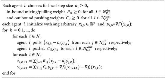
The algebraic form of the push-pull gradient method can be written as:

$x_{k+1}=R\left(x_k-a{y}_k\right),$ (2-7.a)

$y_{k+1}=C{y}_k+\nabla F\left(x_{k+1}\right)-\nabla F\left(x_k\right),$ (2-2.b)

where $a=diag\left\{a_1,a_2,\cdots ,a_n\right\}$ is a non-negative diagonal matrix, and $R=\left[R_{ij}\right],C=\left[C_{ij}\right]R^{n\ast n}$ We derive the hypothesis after this.

Assume 2.2, the matrix $R\in {ℝ}^{n\ast n}$ is non-negative random, and $C\in {ℝ}^{n\ast n}$ is also non-negative random, that is, $R1=1,1^{\text{T}}C=1^{\text{T}}$. In addition, we show that the diagonal terms of R and C are positive, that is, $R_{ii}>0$, $C_{ii}>0$ for $i\in \mathcal{G}$.

Inductive by column random C

$\frac{1}{n}{1}^{\text{T}}{y}_k=\frac{1}{n}{1}^{\text{T}}\nabla F\left(x_k\right),\forall k$ (2-8)

The above relationship has a very important relationship to the average tracking speed of the subset $\frac{1^{\text{T}}\nabla F\left(x_k\right)}{n}$.

Now, we give the graphs ${\mathcal{G}}_R$ and ${\mathcal{G}}_{C^{\text{T}}}$ derived from the matrices R and $C^{\text{T}}$, respectively. Here we want to explain that ${\mathcal{G}}_R$ and ${\mathcal{G}}_{C^{\text{T}}}$ are the same, but all edges are opposite.

Assume 2.3. For graphs ${\mathcal{G}}_R$ and ${\mathcal{G}}_{C^{\text{T}}}$, each contains at least one spanning tree. In addition, at least one node is followed by a spanning tree of ${\mathcal{G}}_R$ and ${\mathcal{G}}_{C^{\text{T}}}$, that is, $R_R\cap R_{C^{\text{T}}}\ne \varnothing$, and $R_R$ is the set of all possible spanning tree roots in graph ${\mathcal{G}}_R$.

For the choice of step size, we assume that at least one node in the range has a positive step size.

From the above prerequisites and assumptions we can get some constraints and the scope of the argument, which intuitively opens the way for the algorithm, so we explain our algorithm from another angle.

In order to show the feasibility of the push-pull algorithm, we first calculate in the optimal form

$x^{*}\in null\left\{I-R\right\},$ (2-9.a)

$1^{\text{T}}\nabla F\left(x^{*}\right)=0$ (2-9.b)

where $x^{*}=1x^{*\text{T}}$, and meet the conditions introduced above, now consider the algorithm proposed above, assuming that the algorithm generates two sequences $\left\{x_k\right\}$ and $\left\{y_k\right\}$, which converge to $x_{\infty }$ and $y_{\infty }$, respectively, We can get

$\left(I-R\right)\left(x_{\infty }-a{y}_{\infty }\right)+a{y}_{\infty }=0,$ (2-10.a)

$\left(I-R\right)y_{\infty }=0.$ (2-10.b)

Here we want to show that if $\left(I-R\right)$ does not intersect the span of $a\cdot null\left\{I-C\right\}$, we will get $x_{\infty }\in null\left\{I-R\right\}$, $a{y}_{\infty }=0$,Therefore, $x_{\infty }$ satisfies

the optimal condition of $x^{*}\in null\left\{I-R\right\}$. From $1\frac{1}{n}{1}^{\text{T}}{y}_k=\frac{1}{n}{1}^{\text{T}}\nabla F\left(x_k\right)$, $1^{\text{T}}\nabla F\left(x^{*}\right)=1^{\text{T}}{y}_{\infty }=0$ is the exactly Optimal condition in $1^{\text{T}}\nabla F\left(x^{*}\right)=0$.

We now reproduce the feasibility of the push-pull algorithm, and from the above assumptions and conditions we know that it is linearly convergent

${\lim }_{k\to \infty }{R}^k=\frac{1u^{\text{T}}}{n},{\lim }_{k\to \infty }{C}^k=\frac{v{1}^{\text{T}}}{n}$ (2-11)

Therefore, in the case of relatively small step sizes, the above relationship means that $x_k\approx \frac{1u^{\text{T}}{x}_{k+1}}{n}$, $y_k\approx \frac{v{1}^{\text{T}}\nabla F\left(x_k\right)}{n}$, $x_k$ means that the entire network

only pulls the state information of the agent $i\in R_R$, while y_k means pushing back the agent $j\in R_{C^{\text{T}}}$ and tracking the average gradient information. This form of “push” and “pull” information gives the name of our proposed algorithm. The information that $R_R\cap R_{C^{\text{T}}}\ne \varnothing$ essentially represents is that at least every agent needs to be pushed and pulled at the same time.

The algorithm in (2-7) is similar in structure to the DIGing algorithm proposed in [44], with mixed matrix distortion. The x update can be viewed as an inexact gradient step with a formula, and it can be viewed as a gradient tracking step. This asymmetric R-C structure design has been used in the literature of average consensus [45], but this algorithm has a gradient term and nonlinear dynamic characteristics, so it cannot explain linear dynamic systems.

Above we have explained the rationality of this method mathematically, now we conceptually explain it as a push-pull algorithm and its reliability. In the current calculation, we still put it in a static network, discuss and analyze it. But in fact, many networks in the real world are dynamic or even unreliable. We need to expand the scope of the discussion. The original algorithm was actually calculated from [44], and it also gave us some inspiration. In a dynamic network, if we need to disseminate or integrate information, we need to know the weight of the scatter or know how to derive its weight. When in an unreliable network, the connection between the dissemination and receiving nodes is not reliable. We need some specific strategies to specify the weight distribution or customization

In order to keep the part of the network we specified converge, a relatively effective method is to make the receiver perform the task of scaling and combining. When the network environment changes, as the underlying sender, it is difficult to know the entire network change and we can adjust the weight accordingly. We can also continue to use the push protocol to communicate and let the surrounding nodes continue to send messages to it. However, it is difficult to determine whether it is still alive (expired) in the network, because we do not know its status should not or cannot respond as death). We can “subjectively” judge whether a certain node or agent is dead. The important reason is that we cannot fully synchronize. If a node waits for a certain period of time without responding, we can consider it to be dead until he again Answer. In fact, a pull communication protocol can also be used to allow agents to pull information from neighbors or nodes for effective coordination and synchronization.

To sum up, for the general implementation of Algorithm 1, the push protocol is indispensable, and using the pull protocol on this basis can improve the network operation efficiency, but it cannot be operated only by the pull network.

2.2. Unify Different Distributed Computing Architecture Systems

We now show how the proposed algorithm unifies different types of distributed architectures to a limited extent. For a completely decentralized case, for example, there is an undirected connection graph $\mathcal{G}$, we can set ${\mathcal{G}}_R={\mathcal{G}}_C=\mathcal{G}$, and let $R=C$, then it becomes a symmetric matrix. In this case, the algorithm can be regarded as [44] [46]. If the graph is directional and closely connected, we can also let ${\mathcal{G}}_R={\mathcal{G}}_C=\mathcal{G}$ and set the corresponding R and C weights.

While it may not be straightforward to implement in a centralized or semi-centralized network, let us illustrate by example. Consider a four-node star network consisting of {1, 2, 3, 4}. Let node 1 be located in the center, and nodes 2, 3, and 4 be connected to node 1. In this case, we can use the matrices R and C are set to

$R=\left[\begin{array}{cccc}1& 0& 0& 0\\ 0.5& 0.5& 0& 0\\ 0.5& 0& 0.5& 0\\ 0.5& 0& 0& 0.5\end{array}\right]$, $C=\left[\begin{array}{cccc}1& 0.5& 0.5& 0.5\\ 0& 0.5& 0& 0\\ 0& 0& 0.5& 0\\ 0& 0& 0& 0.5\end{array}\right]$

As an illustration, Figure 1 shows the network topology diagram of ${\mathcal{G}}_R$ and ${\mathcal{G}}_C$. The central node pushes information such as $x_{1,k}$ to other neighbor nodes through ${\mathcal{G}}_R$. And other nodes or neighbors can only passively wait for the information of the sending node.

At the same time, the node collects information about $y_{i,k}$ from the feedback information through ${\mathcal{G}}_C$, and other nodes can only passively comply with the request from node 1. This very intuitively shows the name of the push-pull algorithm. Although the related nodes 2, 3, and 4 update their information, these numbers do not need to participate in the optimization process. Due to the last three rows of C weights, they are geometrically fast, will disappear. In this case, we can set the local step size of 2, 3, 4 to 0 as a matter of course. In general, we can assume that $f_1\left(x\right)=0,\forall x$, then we can make ${\displaystyle {\sum }_{i=2}^4{f}_i\left(x\right)}$ become a centralized algorithm. The master node uses 2, 3, 4 Calculated by distributed gradient method.

The above example is more of a semi-centralized case. Node 1 cannot be replaced by a strongly connected subnet in R and C, but 2, 3, and 4 can be replaced by different nodes, as long as the information of these subnodes can be passed to ${\mathcal{G}}_R$. In the subordinate agent layer of the above, the theory is discussed in the next section. The layer in ${\mathcal{G}}_C$, using the concept of the root tree, can be understood as the specific requirement of the subnet connectivity. In the network, his role is similar to the role of node 1, we call it the leader, and other nodes are called followers. One thing we want to emphasize here is that a subnet can be used to replace a node, but after the replacement, all subnet structures are decentralized, and the relationship between the leader and the subnet is subordinate. This is what we call a semi-centralized architecture.

Figure 1. Network topology of ${\mathcal{G}}_R$ and ${\mathcal{G}}_C$.

2.3. Proof of Convergence

In this section, we will study the convergence of the algorithm. First, we define ${\bar{x}}_k=\frac{1}{n}{u}^{\text{T}}{x}_k$, ${\bar{y}}_k=\frac{1}{n}{1}^{\text{T}}{y}_k$. Our thinking is based on the linear constraint $\Vert {\bar{x}}_{k+1}\stackrel{\dot{}}{-}{x}^{\star }\Vert$, ${\Vert x_{k+1}\stackrel{\dot{}}{-}1{\bar{x}}_{k+1}\Vert }_R$, ${\Vert y_{k+1}\stackrel{\dot{}}{-}\mathcal{V}{\bar{y}}_{k+1}\Vert }_C$ for binding. Among them, ${\Vert \cdot \Vert }_R$ and ${\Vert \cdot \Vert }_C$ are defined later. He is a specific specification. On this basis, a linear system can be established, which belongs to the inequality.

Algorithm analysis According to Formula (2-7), we can get

${\bar{x}}_{k+1}=\frac{1}{n}{u}^{\text{T}}R\left(x_k\stackrel{\dot{}}{-}\alpha y_k\right)={\bar{x}}_k\stackrel{\dot{}}{-}\frac{1}{n}{u}^{\text{T}}\alpha y_k$ (2-12)

$\begin{array}{c}{\bar{y}}_{k+1}=\frac{1}{n}{1}^{\text{T}}\left(C{y}_k+\nabla F\left(x_{k+1}\right)\cdot \nabla F\left(x_k\right)\right)\\ ={\bar{y}}_k+\frac{1}{n}{1}^{\text{T}}\left(\nabla F\left(x_{k+1}\right)\cdot \nabla F\left(x_k\right)\right)\end{array}$ (2-13)

Let’s further define, $g_k=\frac{1}{n}{1}^{\text{T}}\nabla F\left(1{\bar{x}}_k\right)$,

$a^{\prime }=\frac{1}{n}{u}^{\text{T}}\alpha \mathcal{V}$ (2-14)

From (2-8) and (2-10) we get $a^{\prime }>0$

Then we can get

$\begin{array}{c}{\bar{x}}_{k+1}={\bar{x}}_k\stackrel{\dot{}}{-}\frac{1}{n}{u}^{\text{T}}\left(y_k\stackrel{\dot{}}{-}\mathcal{V}{\bar{y}}_k+\mathcal{V}{\bar{y}}_k\right)\\ ={\bar{x}}_k\stackrel{\dot{}}{-}{a}^{\prime }{g}_k\stackrel{\dot{}}{-}{a}^{\prime }\left({\bar{y}}_k\stackrel{\dot{}}{-}{g}_k\right)\stackrel{\dot{}}{-}\frac{1}{n}{u}^{\text{T}}\alpha \left(y_k\stackrel{\dot{}}{-}\mathcal{V}{\bar{y}}_k\right)\end{array}$ (2-15)

According to the above definition we can get

$\begin{array}{c}{x}_{k+1}\stackrel{\dot{}}{-}1{\bar{x}}_{k+1}=R\left(x_k\stackrel{\dot{}}{-}\alpha y_k\right)\stackrel{\dot{}}{-}1{\bar{x}}_k+\frac{1}{n}{u}^{\text{T}}\alpha y_k\\ =R\left(x_k\stackrel{\dot{}}{-}1{\bar{x}}_k\right)\stackrel{\dot{}}{-}\left(R\stackrel{\dot{}}{-}\frac{1}{n}{u}^{\text{T}}\right)\alpha y_k\\ =\left(R\stackrel{\dot{}}{-}\frac{1}{n}{u}^{\text{T}}\right)\left(x_k\stackrel{\dot{}}{-}1{\bar{x}}_k\right)\stackrel{\dot{}}{-}\left(R\stackrel{\dot{}}{-}\frac{1}{n}{u}^{\text{T}}\right)\alpha y_k\end{array}$ (2-16)

Similarly available

$\begin{array}{c}{y}_{k+1}\stackrel{\dot{}}{-}\mathcal{V}{\bar{y}}_{k+1}=\left(C\stackrel{\dot{}}{-}\frac{1}{n}{1}^{\text{T}}\right)\left(y_k\stackrel{\dot{}}{-}\mathcal{V}{\bar{y}}_k\right)\\ +\left(1\stackrel{\dot{}}{-}\mathcal{V}\frac{1}{n}{1}^{\text{T}}\right)\left(\nabla F\left(x_{k+1}\right)\stackrel{\dot{}}{-}\nabla F\left(x_k\right)\right)\end{array}$ (2-17)

According to $\Vert {\bar{x}}_{k+1}\stackrel{\dot{}}{-}{x}^{\star }\Vert$, ${\Vert x_{k+1}\stackrel{\dot{}}{-}1{\bar{x}}_{k+1}\Vert }_R$, ${\Vert y_{k+1}\stackrel{\dot{}}{-}\mathcal{V}{\bar{y}}_{k+1}\Vert }_C$ lemma we build a linear system of inequality

$\left[\begin{array}{c}\Vert {\bar{x}}_{k+1}\stackrel{\dot{}}{-}{x}^{\star }\Vert \\ {\Vert x_{k+1}\stackrel{\dot{}}{-}1{\bar{x}}_{k+1}\Vert }_R\\ {\Vert y_{k+1}\stackrel{\dot{}}{-}\mathcal{V}{\bar{y}}_{k+1}\Vert }_C\end{array}\right]\le A\left[\begin{array}{c}\Vert {\bar{x}}_k\stackrel{\dot{}}{-}{x}^{\star }\Vert \\ {\Vert x_k\stackrel{\dot{}}{-}1{\bar{x}}_k\Vert }_R\\ {\Vert y_k\stackrel{\dot{}}{-}\mathcal{V}{\bar{y}}_k\Vert }_C\end{array}\right]$

Here the inequality is calculated by component, and the transformation matrix element $A=\left[a_{ij}\right]$ can be obtained

$\left[\begin{array}{c}{a}_{11}\\ a_{21}\\ a_{31}\end{array}\right]=\left[\begin{array}{c}1\stackrel{\dot{}}{-}{a}^{\prime }\mu \\ \hat{a}{\sigma }_R{\Vert \nu \Vert }_{R}L\\ \hat{a}{c}_o{\delta }_{C,2}{\Vert R\Vert }_2{\Vert \upsilon \Vert }_2{L}^2\end{array}\right]$

$\left[\begin{array}{c}{a}_{12}\\ a_{22}\\ a_{32}\end{array}\right]=\left[\begin{array}{c}\frac{\hat{a}L}{\sqrt{n}}\\ {\sigma }_R\left(1+\hat{a}{\Vert \nu \Vert }_R\frac{L}{\sqrt{n}}\right)\\ c_o{\delta }_{C,2}L\left({\Vert R-I\Vert }_2+\hat{a}{\Vert R\Vert }_2{\Vert \upsilon \Vert }_2\frac{L}{\sqrt{n}}\right)\end{array}\right]$

$\left[\begin{array}{c}{a}_{12}\\ a_{22}\\ a_{32}\end{array}\right]=\left[\begin{array}{c}\frac{\hat{a}{\Vert u\Vert }_2}{\sqrt{n}}\\ \hat{a}{c}_R{\delta }_{R,C}\\ {\sigma }_C+\hat{a}{c}_o{\delta }_{C,2}{\Vert R\Vert }_2{L}^2\end{array}\right]$

It’s here $\hat{a}=\max a_i$, $c_o={\Vert I-\upsilon \frac{1}{n}{1}^{\text{T}}\Vert }_C$.

According to the previous inequality linear system, we know that when the spectral radius $\rho \left(A\right)<1$ is satisfied, $\Vert {\bar{x}}_{k+1}\stackrel{\dot{}}{-}{x}^{\star }\Vert$, ${\Vert x_{k+1}\stackrel{\dot{}}{-}1{\bar{x}}_{k+1}\Vert }_R$, ${\Vert y_{k+1}\stackrel{\dot{}}{-}\mathcal{V}{\bar{y}}_{k+1}\Vert }_C$ converge to 0 at a linear rate ℴ $\left(\rho {\left(A\right)}^k\right)$. The problem to be explained next is $\rho \left(A\right)<1$.

Given a nonnegative irreducible matrix $M=\left[m_{ij}\right]\in {ℝ}^{3\ast 3}$, $i=1,2,3$ and $m_{ij}<{\lambda }^{*}$, then $\rho \left(M\right)<{\lambda }^{*}$ is $\left({\lambda }^{*}I-M\right)>0$ Necessary and sufficient conditions.

We now give convergence results for the proposed algorithm.

We assume that in the algorithm (1-1), $M>0$ in $a^{\prime }\ge M\hat{a}$, we get

$\hat{a}\le \min \left\{\frac{2c_3}{c_2+\sqrt{c_2^2+4c_1{c}_3}},\frac{\left(1-{\sigma }_C\right)}{2{\sigma }_C{\delta }_{C,2}{\Vert R\Vert }_{2}L}\right\}$ (2-18)

Among them $c_1,c_2,c_3$ will be given later. In this way, when the spectral radius $\rho \left(A\right)<1$ is satisfied, $\Vert {\bar{x}}_{k+1}\stackrel{\dot{}}{-}{x}^{\star }\Vert$, ${\Vert x_{k+1}\stackrel{\dot{}}{-}1{\bar{x}}_{k+1}\Vert }_R$, ${\Vert y_{k+1}\stackrel{\dot{}}{-}\mathcal{V}{\bar{y}}_{k+1}\Vert }_C$ converges to 0 at a linear rate ℴ $\left(\rho {\left(A\right)}^k\right)$.

We prove that according to the above lemma, we guarantee that $a_{11},a_{22},a_{33}<1$, and

$\begin{array}{l}\det \left(I-A\right)\\ =\left(1-a_{11}\right)\left(1-a_{22}\right)\left(1-a_{33}\right)-a_{23}{a}_{31}-a_{13}{a}_{21}{a}_{32}\\ -\left(1-a_{22}\right)a_{13}{a}_{31}-\left(1-a_{11}\right)a_{23}{a}_{32}-\left(1-a_{11}\right)a_{12}{a}_{21}\\ =\left(1-a_{11}\right)\left(1-a_{22}\right)\left(1-a_{33}\right)-a^{\prime }{\hat{a}}^2{\sigma }_R{c}_o{\delta }_{R,C}{\delta }_{2,C}{\Vert R\Vert }_2{\Vert v\Vert }_2\frac{L^3}{\sqrt{n}}\\ -{\hat{a}}^2{\sigma }_R{c}_o{\delta }_{2,C}{\Vert u\Vert }_2{\Vert v\Vert }_R\left({\Vert R-I\Vert }_2+\hat{a}{\Vert R\Vert }_2{\Vert v\Vert }_2\frac{L}{\sqrt{n}}\right)\frac{L^2}{\sqrt{n}}\end{array}$

$\begin{array}{l}-{\hat{a}}^2{c}_o{\delta }_{2,C}{\Vert R\Vert }_2{\Vert v\Vert }_2{\Vert u\Vert }_2\frac{L^2}{\sqrt{n}}\left(1-a_{22}\right)\\ -\hat{a}{\sigma }_R{c}_o{\delta }_{R,C}{\delta }_{2,C}L\left({\Vert R-I\Vert }_2+\hat{a}{\Vert R\Vert }_2{\Vert v\Vert }_2\frac{L}{\sqrt{n}}\right)\left(1-a_{11}\right)\\ -a^{\prime }\hat{a}{\sigma }_R{\Vert v\Vert }_2\frac{L^2}{\sqrt{n}}\left(1-a_{33}\right)>0\end{array}$ (2-19)

The small problem now is to explain that $a_{11},a_{22},a_{33}<1$ make the above formula hold.

First, $a_{11}<1$, $1-a_{22}\ge \frac{\left(1-{\sigma }_R\right)}{2}$ and $1-a_{33}\ge \frac{\left(1-{\sigma }_C\right)}{2}$ are guaranteed in the selected $a^{\prime }\le \frac{2}{\left(\mu +L\right)}$, we can get

$\hat{a}\le \min \left\{\frac{\left(1-{\sigma }_C\right)\sqrt{n}}{2{\sigma }_R{\Vert v\Vert }_{R}L},\frac{\left(1-{\sigma }_C\right)}{2c_o{\delta }_{C,2}{\Vert R\Vert }_{2}L}\right\}$ (2-20)

Secondly, the sufficient condition for making $\det \left(I-A\right)>0$ is to replace $\left(1-a_{11}\right)$ with $\left(1-{\sigma }_C\right)/2$, and the rest is similar, so that $a^{\prime }=M\hat{a}$. We can get $c_1{\hat{a}}^2+c_2\hat{a}-c_3<0$.

Here we explain $c_1,c_2,c_3$

$\begin{array}{c}{c}_1=M{\sigma }_R{c}_o{\delta }_{C,2}{\delta }_{R,C}{\Vert R\Vert }_2{\Vert v\Vert }_2\frac{L^3}{\sqrt{n}}+M\mu {\sigma }_R{c}_o{\delta }_{C,2}{\delta }_{R,C}{\Vert R\Vert }_2{\Vert v\Vert }_2\frac{L^2}{\sqrt{n}}\\ +{\sigma }_R{c}_o{\delta }_{C,2}{\Vert R\Vert }_2{\Vert v\Vert }_R{\Vert u\Vert }_2\frac{L^3}{n\sqrt{n}}\\ ={\sigma }_R{c}_o{\delta }_{C,2}{\Vert R\Vert }_2{\Vert v\Vert }_2\frac{L^2}{n\sqrt{n}}\left[M{\delta }_{R,C}n\left(L+\mu \right)+{\Vert v\Vert }_R{\Vert u\Vert }_{2}L\right]\end{array}$ (2-21)

get

$\begin{array}{c}{c}_2={\sigma }_R{c}_o{\delta }_{C,2}{\Vert R\Vert }_2{\Vert v\Vert }_R{\Vert u\Vert }_2{\Vert R-I\Vert }_2\frac{L^2}{n}\\ +c_o{\delta }_{C,2}{\Vert R\Vert }_2{\Vert v\Vert }_R{\Vert u\Vert }_2\left(1-{\sigma }_C\right)\frac{L^2}{2n}\\ +M{\sigma }_R{c}_o{\delta }_{C,2}{\delta }_{R,C}\mu {\Vert R-I\Vert }_{2}L+\frac{{\sigma }_R}{2}M\left(1-{\sigma }_C\right){\Vert v\Vert }_R\frac{L^2}{\sqrt{n}}\end{array}$ (2-22)

And then

$c_3=M\frac{\left(1-{\sigma }_C\right)\left(1-{\sigma }_R\right)}{4}\mu$ (2-23)

As discussed above

$\hat{a}\le \frac{2c_3}{c_2+\sqrt{c_2^2+4c_1{c}_3}}$ (2-24)

From this we get the final limit of $\hat{a}$.

3. Finite-Time Convergence Algorithm

Now we introduce the optimization algorithm for finite-time convergence. Compared with most existing distributed convex optimization algorithms that can only achieve exponential convergence, this algorithm can achieve finite-time convergence. The convergence of the algorithm can be guaranteed by Lyapunov’s finite-time stability theory.

3.1. Algorithm Introduction

Consider a network with N nodes. Each node on the network has its own cost function, expressed as $f_i:{ℝ}^{+}\to ℝ$, which is strictly convex. All nodes cooperate to obtain the optimal value of the target cost function. In order to better design the algorithm, we give the following assumptions:

Assumption 3.1: The upper-layer communication topology network is undirected and connected.

Assumption 3.2: For each proxy node $i\in \mathcal{V}$ of the network, his cost function $f_i$ is second-order continuously differentiable strongly convex, the convex parameter ${\theta }_i>0$, and the Hessian matrix ${\nabla }^2{f}_i$ meets the local Lipschitz condition.

From this we get

$\{\begin{array}{l}{x}_i\left(t\right)=\gamma {\left({\nabla }^2{f}_i\left(x_i\left(t\right)\right)\right)}^{-1}{\displaystyle {\sum }_{j\in {\mathcal{N}}_i}{a}_{ij}Sig{\left|x_j\left(t\right)-x_i\left(t\right)\right|}^a}\\ x_i\left(0\right)=x_i^{*},\forall i\in \mathcal{V}\end{array}$ (3-1)

where $x_i\in {ℝ}^n$ represents the state of node i, and $\gamma \in {ℝ}^{+}$ is a gain constant that can be used to improve the convergence speed of Aijie; $N_i=\left\{j\in \mathcal{V}:\left(i,j\right)\in \mathcal{E}\left(\mathcal{G}\right)\right\}$ means The set of all neighbor nodes of node i; $a_{ij}$ is an element of the adjacency matrix A; $0<a<1$.

And $x_i^{*}$ is the optimal value of cost function $f_i$.

Note 3.1: The algorithm (3-1) is inspired by continuous time zero gradient [10] and finite time consistency protocol [20]. From the first formula,

$\frac{\text{d}}{\text{d}t}{\displaystyle \underset{i\in \mathcal{V}}{\sum }\nabla f_i\left(x_i\left(t\right)\right)}={\displaystyle \underset{i\in \mathcal{V}}{\sum }\left({\nabla }^2{f}_i\left(x_i\left(t\right)\right)\right)x_i\left(t\right)}={\displaystyle \underset{i\in \mathcal{V}}{\sum }{\displaystyle \underset{i\in \mathcal{V}}{\sum }{a}_{ij}Sig{\left|x_j\left(t\right)-x_i\left(t\right)\right|}^a}}=0$.

From the second formula, we can get ${\displaystyle {\sum }_{i\in \mathcal{V}}\nabla f_i\left(x_i\left(0\right)\right)}=0$, So it is easy to get the gradient and satisfy

${\displaystyle {\sum }_{i\in \mathcal{V}}\nabla f_i\left(x_i\left(t\right)\right)}=0,\forall i\ge 0$

where ${\displaystyle {\sum }_{j\in {\mathcal{N}}_i}{a}_{ij}Sig{\left|x_j\left(t\right)-x_i\left(t\right)\right|}^a}$ can ensure that the algorithm achieves finite-time consistent convergence, that is, there is a convergence time T and a convergence state $\tilde{x}$. For $\forall i\in \mathcal{V}$, both have ${\lim }_{t\to T}{x}_i\left(t\right)=\tilde{x}$ and ${\displaystyle {\sum }_{i\in \mathcal{V}}\nabla f_i\left(\tilde{x}\right)}=\nabla F\left(\tilde{x}\right)=0$. From the hypothesis 2, we know that $F\left(x\left(t\right)\right)$ Strongly convex has only one optimal value $x^{*}$, and satisfies $\nabla F\left(x^{*}\right)={\displaystyle {\sum }_{i\in \mathcal{V}}\nabla f_i\left(x^{*}\right)}=0$. The above analysis shows that $\tilde{x}=x^{*}$, which shows that at the upper level, this algorithm can solve the problem we raised. It should be noted that when $\alpha =1$, the algorithm only achieves progressive convergence.

3.2. Convergence Analysis

Theorem 3.1: Based on assumptions 1 and 2, our proposed algorithm can solve the target problem in a finite time, and the bound of its convergence time is T. It also shows that ${\lim }_{t\to T}x\left(t\right)=x^{*}$ Where T satisfies:

$T\le \frac{4V^{\frac{1-a}{2}}\left(\tilde{x}\left(t_0\right)\right)}{\gamma \left(1-a\right){\left(\frac{4{\lambda }_2}{\Theta }\right)}^{\frac{1+a}{2}}}$ (3-2)

Among them $x\left(t\right)={\left(x_1{\left(t\right)}^{\text{T}},x_2{\left(t\right)}^{\text{T}},\cdots ,x_N{\left(t\right)}^{\text{T}}\right)}^{\text{T}}\in {ℝ}^{nN}$ ;

$x^{*}={\left(x^{*\text{T}},x^{*\text{T}},\cdots ,x^{*\text{T}}\right)}^{\text{T}}$ ; $x\left(t_0\right)={\left(x_1^{*\text{T}},x_2^{*\text{T}},\cdots ,x_N^{*\text{T}}\right)}^{\text{T}}$, $V\left(x\right)$ is a continuous positive definite Lyapunov function, ${\lambda }_2$ is the algebraic connectivity related to the topological graph, and $\Theta >0$ is a constant related to $f_i\left(i\in \mathcal{V}\right)$.

Proof: This part of the Lyapunov method gives a proof of Theorem 3.1. First,

$V\left(x\left(t\right)\right)={\displaystyle {\sum }_{i\in V}{f}_i\left(x^{*}\right)}-f_i\left(x_i\left(t\right)\right)-\nabla f_i{\left(x_i\left(t\right)\right)}^{\text{T}}\left(x^{*}-x_i\left(t\right)\right)$ (3-3)

This function is given in [10]. Based on Hypothesis 3.2, $V\left(x\left(t\right)\right)$ is a second-order continuously differentiable function. It is also known that $V\left(x\left(t\right)\right)$ is a locally strongly convex function.

Next, for convenience of derivation, we give the following definitions:

For $i\in V$, $f_i$ is a local strongly convex function. From the above formula, we know that $U_i$ is a compact set. In order to take advantage of the strong convex function, we need to find another convex compact set, so we let $U=conv\left(U_{i\in \mathcal{V}}{U}_i\right)$, where “ $conv$ “ represents a convex set From hypothesis 3.2, we can know that $U_i\left(i\in \mathcal{V}\right)$ is a compact set, U is a convex compact set and satisfies $\forall t\ge 0,\forall i\in \mathcal{V},x^{*}\in U_i\subset U$ is based on the convex compact set U, for every $i\in \mathcal{V}$, combined with hypothesis 3.2, there will be ${\Theta }_i\ge {\theta }_i$ satisfying

${\displaystyle {\sum }_{i\in \mathcal{V}}\frac{{\Theta }_i}{2}{\Vert x^{*}-x_i\left(t\right)\Vert }^2}\ge V\left(x\left(t\right)\right)\ge {\displaystyle {\sum }_{i\in \mathcal{V}}\frac{{\theta }_i}{2}{\Vert x^{*}-x_i\left(t\right)\Vert }^2},x\left(t\right)\in U$ (3-5)

From (3-5), we can get V $V\left(x\left(t\right)\right)\ge 0$, when $\forall x\left(t\right)\in U$. Considering the derivative of V with respect to time, then for $\forall x\left(t\right)\in U$, the following relationship exists

$V\left(x\left(t\right)\right)=\frac{\gamma }{2}{\displaystyle {\sum }_{i\in \mathcal{V}}{\displaystyle {\sum }_{j\in N_i}{\left(x_j\left(t\right)-x_i\left(t\right)\right)}^{\text{T}}{\phi }_{ij}}}$ (3-6)

where ${\phi }_{ij}=a_{ij}Sig{\left|x_j\left(t\right)-x_i\left(t\right)\right|}^a$, we can get ${\left(x_j\left(t\right)-x_i\left(t\right)\right)}^{\text{T}}{\phi }_{ij}\ge {\Vert x_j\left(t\right)-x_i\left(t\right)\Vert }^{\left(a+1\right)}\ge 0,V\le 0$ if and only if the equation $x\left(t\right)=x^{*}$ holds, so V can be used to prove Theorem 3.1.

In addition, $\frac{\text{d}}{\text{d}t}\underset{i\in \mathcal{V}}{{\displaystyle \sum }}\nabla f_i\left(x_i\left(t\right)\right)=\underset{i\in \mathcal{V}}{{\displaystyle \sum }}\left({\nabla }^2{f}_i\left(x_i\left(t\right)\right)\right)x_i\left(t\right)=\gamma \underset{i\in \mathcal{V}}{{\displaystyle \sum }}\underset{ij\in N_i}{{\displaystyle \sum }}{\phi }_{ij}=0$, combining the existing initial conditions, we can get the following properties ${\displaystyle {\sum }_{i\in \mathcal{V}}\nabla f_i\left(x_i\left(t\right)\right)}=0$. We set $\eta \left(t\right)=\frac{1}{N}{\displaystyle {\sum }_{i\in \mathcal{V}}{x}_i\left(t\right)}\in U$, there are $F\left(x^{*}\right)\le F\left(\eta \left(t\right)\right)$ And can get the following inequality

$V\left(x\left(t\right)\right)\le {\displaystyle {\sum }_{i\in \mathcal{V}}F\left(\eta \left(t\right)\right)-f_i\left(x_i\left(t\right)\right)-\nabla f_i{\left(x_i\left(t\right)\right)}^{\text{T}}\left(\eta \left(t\right)-x_i\left(t\right)\right)}$ (3-7)

Combining (1-4) for $x\left(t\right)\in U$, (3-7) can be written as

$V\left(x\left(t\right)\right)\le {\displaystyle {\sum }_{i\in \mathcal{V}}\frac{{\Theta }_i}{2}{\Vert x_i\left(t\right)-\frac{1}{N}{\displaystyle {\sum }_{j\in \mathcal{V}}{x}_i\left(t\right)}\Vert }^2}=\frac{{\Theta }_i}{2N}x{\left(t\right)}^{\text{T}}\left(\mathcal{L}\left(\bar{\mathcal{G}}\right)\otimes I_n\right)x\left(t\right),$ (3-8)

where $\Theta =\max {\left\{{\Theta }_i\right\}}_{i\in \mathcal{V}}$, $\bar{\mathcal{G}}$ is the complete graph of graph $\mathcal{G}$, then combining Cauchy's inequality and (3-6), we can get

$\begin{array}{c}V\left(x\left(t\right)\right)\le -\frac{\gamma }{2}{\displaystyle {\sum }_{i\in \mathcal{V}}{\displaystyle {\sum }_{j\in N_i}{\left[{\Vert x_j\left(t\right)-x_i\left(t\right)\Vert }^2\right]}^{\frac{a+1}{2}}}}\\ \le -2\frac{a-1}{2}\gamma {\left\{\frac{1}{2}{\displaystyle {\sum }_{i\in \mathcal{V}}{\displaystyle {\sum }_{j\in N_i}{\Vert x_j\left(t\right)-x_i\left(t\right)\Vert }^2}}\right\}}^{\frac{a+1}{2}}\\ =-2\frac{a-1}{2}\gamma {\left(x{\left(t\right)}^{\text{T}}\left(\mathcal{L}\left(\bar{\mathcal{G}}\right)\otimes I_n\right)x\left(t\right)\right)}^{\frac{a+1}{2}}\end{array}$ (3-9)

Due to ${\lambda }_2\left(x{\left(t\right)}^{\text{T}}\left(\mathcal{L}\left(\bar{\mathcal{G}}\right)\otimes I_n\right)x\left(t\right)\right)\le N\left(x{\left(t\right)}^{\text{T}}\left(\mathcal{L}\left(\bar{\mathcal{G}}\right)\otimes I_n\right)x\right)\left(t\right)$, Combining (3-8) we get:

$V\left(x\left(t\right)\right)\le -\frac{\gamma }{2}{\left(\frac{4{\lambda }_2}{\Theta }\right)}^{\frac{a+1}{2}}V{\left(x\left(t\right)\right)}^{\frac{a+1}{2}}$ (3-10)

Combined with the finite-time stability theorem proposed earlier, we can get that our algorithm is convergent, then there is a time T, ${\lim }_{t\to T}V\left(x\left(t\right)\right)=0$ $V\left(x\left(t\right)\right)\equiv 0\left(t>T\right)$. That is ${\lim }_{t\to T}V\left(x\left(t\right)\right)=x^{*}$, In addition, the bound of T

can be obtained from Theorem (3.1) $T\le \frac{4V^{\frac{1-a}{2}}\left(\tilde{x}\left(t_0\right)\right)}{\gamma \left(1-a\right){\left(\frac{4{\lambda }_2}{\Theta }\right)}^{\frac{a+1}{2}}}$. Among them, the

convergence speed is related to parameters such as algebraic connectivity ${\lambda }_2$, function curvature $\Theta ,f_i,\gamma ,\alpha$, etc.

3.3. Simulation

In this section, a simulation experiment is given to demonstrate the effectiveness of the algorithm in this section. We set up a 6-node network topology diagram, as shown in Figure 2. His adjacency matrix is $A_1=\left[a_{ij}\right]$ and $A_2=\left[a_{ij}\right]$. The cost function of each node is

$f_i\left(x\right)=\frac{1}{8}{\left(x-i\right)}^6+\frac{3}{4}{\left(x-i\right)}^2,i=1,2,\cdots ,6.$ (3-11)

It can be obtained that the optimal value of each node satisfies $x_i^{*}=i$, $i\in \left\{1,2,\cdots ,6\right\}$. The optimal value of Equation (1-1) is calculated as $x^{*}=3.5$, $V\left(x\left(0\right)\right)=130.168$. Combining the convex compact set U in the proof, we can get ${\Theta }_1=41.6538$, ${\Theta }_2=115.7049$, ${\Theta }_3=1041.3$, ${\Theta }_4=1041.3$, ${\Theta }_5=115.7049$, ${\Theta }_6=41.6538$, which means $\Theta =1041.3$.

In the simulation, we use the parameter values ${\lambda }_2\left({\mathcal{G}}_1\right)=0.5858$, $\alpha =0.5$, $\gamma =10$, and the simulation results are shown in Figure 3.

Figure 2. Six-node network topology.

Figure 3. ${\lambda }_2\left({\mathcal{G}}_1\right)=0.5858,\alpha =0.5,\gamma =10$.

4. Push-Pull Fast Convergent Distributed Cooperative Learning Algorithm

This chapter aims to combine and generalize the previously proposed algorithms to practical applications, such as common machine learning scenarios. Inspired by the previous algorithm, we will design a fast convergent distributed cooperative learning (P-DCL) algorithm based on a linear parameterized neural network based on push-pull mode. In the first step, a P-DCL algorithm based on continuous-time convergence in push-pull gradient mode is first given. In the second step, we give a convergence analysis of the algorithm based on the Lyapunov method. In the third step, for the practical effect of the algorithm, we use the fourth-order Runge-Kutta (RK4) method to discretize the algorithm. In the fourth step, the distributed ADMM algorithm and the push-pull gradient-based (P-DCL) algorithm simulation are given. Experiments show that our proposed algorithm has higher learning ability and faster convergence speed. Finally, we give the relationship between the algorithm’s own convergence speed and some parameters. Simulation results show that the convergence speed of the algorithm can be effectively improved by properly selecting some adjustable parameters.

Restatement: In order to construct the algorithm systematically, the problem formation is given first, and then the local cost function is analyzed. Then the relationship between global cost function and local cost function solution is given.

Consider a network with N nodes. Each node $i\in \mathcal{V}$ in the network contains $M_i\in {ℝ}^{+}$ samples, and each sample set can be expressed as $D_i=U_{k=1}^{M_i}\left\{X_i^{\left(k\right)}{Y}_i^{\left(k\right)}\right\}$, Where $\left\{X_i^{\left(k\right)}{Y}_i^{\left(k\right)}\right\}$, represents the k-th sample on the i-th node, so for each node, their local cost function can be expressed as:

$E_i^{loc}\left(W_i\right)\triangleq \frac{1}{2}{\Vert Y_i-S\left(Y_i\right)W_i\Vert }_2^2+\frac{{\delta }_i}{2}{\Vert W_i\Vert }_2^2$ (4-1)

$W_i\in {ℝ}^{l\times n}$ is the learning weight of the i-th node, $X_i\in {ℝ}^{M_i\times m}$ represents the sample of the i-th node; $Y_i$ and $S\left(Y_i\right)W_i$ represent the expectations of With the output, ${\delta }_i$ is a non-negative constant. In this way, the optimal learning weight of node i can be easily obtained.

$W_i^{*}={\left(S{\left(X_i\right)}^{\text{T}}S\left(X_i\right)+{\delta }_i{I}_l\right)}^{-1}S{\left(X_i\right)}^{\text{T}}{Y}_i$ (4-2)

If all the node samples satisfy ${\displaystyle {\sum }_{i=1}^N{M}_i}=M$, the adjustment parameters of all nodes satisfy ${\displaystyle {\sum }_{i=1}^N{\delta }_i}=K$. Then the W-optimal global cost function (1-7) is equivalent to the sum function of the local cost functions of each node.

$E^{glob}\left(W\right)={\displaystyle {\sum }_{i=1}^N{E}_i^{loc}\left(W\right)}$ (4-3)

As mentioned earlier, there are many distributed solving algorithms for this problem that can achieve progressive convergence. Next, what needs to be done is to design a fast distributed optimization algorithm, such as the following requirements:

${\lim }_{t\to T}{W}_i\to W^{*},i\in \left\{1,\cdots ,N\right\}$ (4-4)

This shows that all nodes can converge to the optimal learning weight $W^{*}$ in a finite time T.

From the above analysis, the global cost function (1-7) can be written as:

$\{\begin{array}{l}\min {\displaystyle {\sum }_{i=1}^N{E}_i\left(W_i\right)}\\ \text{s}\text{.t}\text{.}{W}_i-W^{*}=0,i=1,\cdots ,N\end{array}$ (4-5)

This is often referred to as global consistency. Unlike the traditional multi-agent consistency problem, the result of consistency convergence here has no specific meaning. Consistency has a long history of research. The basic concept is that all nodes in all networks eventually reach the same state through information exchange with neighbors. From the perspective of learning, an efficient learning algorithm is very necessary. For distributed cooperative learning algorithms, their learning rate is an important measurement index of their algorithm. However, in real life, it is more necessary to reach a valid result within a certain time, which also prompts us to design a fast consensus learning cooperation algorithm.

4.1. Fast Convergent Distributed Algorithm

Here, based on the linear parameterized neural network, a distributed strategy for the target problem is given. To build a better construction algorithm, the following assumptions are given first:

Hypothesis 4.1 assumes that the network topology $\mathcal{G}$ is undirected and connected.

Based on the previous analysis, the distributed cooperative learning algorithm in continuous time gives:

$\{\begin{array}{l}{W}_i\left(t\right)=\rho {\left(S{\left(X_i\right)}^{\text{T}}S\left(X_i\right)+{\delta }_i{I}_l\right)}^{-1}{\displaystyle {\sum }_{j\in N_i}Sig{\left|W_j\left(t\right)-W_i\left(t\right)\right|}^{\beta }},\\ W_i\left(t_0\right)={\left(S{\left(X_i\right)}^{\text{T}}S\left(X_i\right)+{\delta }_i{I}_l\right)}^{-1}S{\left(X_i\right)}^{\text{T}}{Y}_i\end{array}$ (4-6)

where $\rho \in R^{+}$ is a constant used to adjust the convergence rate. $0<\beta <1$, $a_{i,j}$ is an element in the adjacency matrix $\mathcal{A}$ ; $Sig{\left|W_j\left(t\right)-W_i\left(t\right)\right|}^{\beta }=Sig\left(W_j\left(t\right)-W_i\left(t\right)\right)\odot {\left|W_j\left(t\right)-W_i\left(t\right)\right|}^{\beta }$, Figure 4 can show the operation of the algorithm more intuitively.

Let $\tilde{W}\left(t\right)={\left[W{\left(t\right)}_1^{\text{T}},W{\left(t\right)}_2^{\text{T}},\cdots ,W{\left(t\right)}_N^{\text{T}}\right]}^{\text{T}}\in {ℝ}^{lN\times n}$, $Q\left(X\right)=diag\left[S\left(X_1\right),S\left(X_2\right),\cdots ,S\left(X_N\right)\right]\in {ℝ}^{M\times lN}$, $\Delta =diag\left({\delta }_1{I}_l,{\delta }_2{I}_l,\cdots ,{\delta }_N{I}_l\right)$, The algorithm can be written as a matrix:

$\{\begin{array}{l}\tilde{W}\left(t\right)=\rho {\left(Q{\left(X\right)}^{\text{T}}Q\left(X\right)+\Delta I_{lN}\right)}^{-1}Sig\left(\left(-\mathcal{L}\otimes I_l\right)\tilde{W}\left(t\right)\right)\odot {\left|\left(\mathcal{L}\otimes I_l\right)\tilde{W}\left(t\right)\right|}^{\beta }\\ \beta \tilde{W}\left(t_0\right)={\left(Q{\left(X\right)}^{\text{T}}Q\left(X\right)+\Delta \right)}^{-1}Q{\left(X\right)}^{\text{T}}Y\end{array}$ (4-7)

Note 4.1: The above algorithms are inspired by [47]. Linear consistency algorithms can achieve progressive convergence, while cruise ship consistency algorithms that can achieve limited time convergence mostly use symbolic functions [20] [39]. $\frac{\text{d}}{\text{d}t}{\displaystyle {\sum }_{i\in \mathcal{V}}\nabla E_i\left(W_i\left(t\right)\right)}={\displaystyle {\sum }_{i\in \mathcal{V}}{\displaystyle {\sum }_{i\in {\mathcal{N}}_i}{a}_{ij}Sig{\left|W_j\left(t\right)-W_i\left(t\right)\right|}^{\beta }}}=0$, by setting $W_i\left(0\right)=W_i^{*}$, there is ${\displaystyle {\sum }_{i\in \mathcal{V}}\nabla E_i\left(W_i\left(t\right)\right)}=0$, so it is easy to get the gradient sum of the node cost function Satisfies ${\displaystyle {\sum }_{i\in \mathcal{V}}\nabla E_i\left(W_i\left(t\right)\right)}\equiv 0,\forall t\ge 0$, and because $E\left(W\left(t\right)\right)$ is a strong convex function, that is, it has only one optimal. The value also reflects that the algorithm we mentioned does have a solution.

Theorem 4.1: The algorithm (4-7) can achieve the goal in a finite time T, where time T satisfies:

Figure 4. Algorithm (4-6) running on i-node.

$T\le \frac{4V^{\frac{1-\beta }{2}}\left(\tilde{W}\left(t_0\right)\right)}{\rho \left(1-\beta \right){\left(\frac{4{\lambda }_2}{\Theta }\right)}^{\frac{1+\beta }{2}}}$ (4-8)

where $V\left(\tilde{W}\left(t_0\right)\right)$ is a second-order continuous positive definite function, $\beta$ is a constant in the algorithm (4-7), $\tilde{W}\left(t_0\right)=\left[W_1^{*};\cdots ;W_N^{*}\right]$ ; ${\lambda }_2$ is related to the network topology Graph-related algebraic connectivity. $\Theta$ is a constant related to the cost function of all nodes; $\rho$ is the gain constant in the algorithm.

Proof: Based on the Lyapunov method, a rigorous proof of Theorem 4.1 is given next. Before certification, some related work needs to be prepared. First, select:

$\begin{array}{c}V\left(\tilde{W}\left(t\right)\right)=\frac{1}{2}{\displaystyle {\sum }_{i\in \mathcal{V}}{\left(W^{*}-W_i\left(t\right)\right)}^{\text{T}}{\nabla }^2{E}_i\left(W_i\left(t\right)\right)\left(W^{*}-W_i\left(t\right)\right)}\\ =\frac{1}{2}{\displaystyle {\sum }_{i\in \mathcal{V}}{\left(W^{*}-W_i\left(t\right)\right)}^{\text{T}}\left(S{\left(X_i\right)}^{\text{T}}S\left(X_i\right)+{\delta }_i{I}_l\right)\left(W^{*}-W_i\left(t\right)\right)}\end{array}$ (4-9)

As a Lyapunov candidate function, $V:{ℝ}^{lnN}\to ℝ$. Since $\left(S{\left(X_i\right)}^{\text{T}}S\left(X_i\right)+{\delta }_i{I}_l\right)>0$, then we can get $V\left(\tilde{W}\left(t\right)\right)>0,\forall \tilde{W}\left(t\right)\ne W^{*}$, change In other words, $V\left(\tilde{W}\left(t\right)\right)$ in the Formula (4-9) is positive definite. In addition,

$\begin{array}{c}V\left(\tilde{W}\left(t\right)\right)={\displaystyle {\sum }_{i\in \mathcal{V}}{\left(W^{*}-W_i\left(t\right)\right)}^{\text{T}}-\nabla E_i{\left(W_i\left(t\right)\right)}^{\text{T}}\left(W^{*}-W_i\left(t\right)\right)}\\ \le {\displaystyle {\sum }_{i\in \mathcal{V}}{E}_i\left(\eta \left(t\right)\right)-E_i\left(W_i\left(t\right)\right)-\nabla E_i{\left(W_i\left(t\right)\right)}^{\text{T}}-\left(\eta \left(t\right)-W_i\left(t\right)\right)}\end{array}$,

where $\eta \left(t\right)=\frac{1}{N}{\displaystyle {\sum }_{i\in \mathcal{V}}{W}_i\left(t\right)}$, then:

$\begin{array}{c}V\left(\tilde{W}\left(t\right)\right)\le {\displaystyle {\sum }_{i\in \mathcal{V}}\frac{{\Theta }_i}{2}{\Vert W_i\left(t\right)-\frac{1}{N}{\displaystyle {\sum }_{j\in \mathcal{V}}{W}_j\left(t\right)}\Vert }^2}\\ =\frac{\Theta }{2N}W{\left(t\right)}^{\text{T}}\left(\mathcal{L}\left(\tilde{\mathcal{G}}\right)\otimes I_n\right)W\left(t\right),\end{array}$ (4-10)

where ${\Theta }_i={\lambda }_{\max }\left({\nabla }^2{E}_i\left(W_i\left(t\right)\right)\right)$, $\Theta =\max {\left\{{\Theta }_i\right\}}_{i\in \mathcal{V}}$, $\mathcal{L}\left(\mathcal{G}\right)$, $\mathcal{L}\left(\mathcal{G}\right)$ is the Laplacian matrix of $\mathcal{G}$, and $\tilde{\mathcal{G}}$ is completely Figure of $\mathcal{G}$.

Next, by calculating the inverse of $V\left(\tilde{W}\left(t\right)\right)$, we can get

$\begin{array}{c}V\left(\tilde{W}\left(t\right)\right)=-{\displaystyle {\sum }_{i\in \mathcal{V}}}{\left(W^{*}-W_i\left(t\right)\right)}^{\text{T}}\left(S{\left(X_i\right)}^{\text{T}}S\left(X_i\right)+{\delta }_i{I}_l\right)W_i\left(t\right)\\ =W^{*}{\displaystyle {\sum }_{i\in \mathcal{V}}{\displaystyle {\sum }_{i\in N_i}{\phi }_{ij}}}+{\displaystyle {\sum }_{i\in \mathcal{V}}{W}_i{\left(t\right)}^{\text{T}}}{\displaystyle {\sum }_{i\in N_i}{\phi }_{ij}}\end{array}$ (4-11)

where $N_i=\left\{j\in \mathcal{V}:\left(i,j\right)\in \epsilon \left(\mathcal{G}\right)\right\}$ represents the neighbor of node i, ${\phi }_{ij}=a_{ij}sig\left(W_j\left(t\right)-W_i\left(t\right)\right)\odot {\left|W_j\left(t\right)-W_i\left(t\right)\right|}^{\beta }$, we can get ${\phi }_{ij}=-{\phi }_{ij}$, which also means

${\displaystyle {\sum }_{i\in \mathcal{V}}{\displaystyle {\sum }_{i\in N_i}{\phi }_{ij}}}=0$ (4-12)

In addition, it can be concluded

$\begin{array}{c}{\displaystyle {\sum }_{i\in \mathcal{V}}{W}_i{\left(t\right)}^{\text{T}}}{\displaystyle {\sum }_{i\in N_i}{\phi }_{ij}}=-\frac{\rho }{2}{\displaystyle {\sum }_{i\in \mathcal{V}}{\displaystyle {\sum }_{i\in N_i}{\left(W_j\left(t\right)\right)}^{\text{T}}}}-W_i\left(t\right){\phi }_{ij}\\ \le -\frac{\rho }{2}{\displaystyle {\sum }_{i\in \mathcal{V}}{\displaystyle {\sum }_{i\in N_i}{\Vert W_j\left(t\right)-W_i\left(t\right)\Vert }^{\left(\beta +1\right)}}}\end{array}$ (4-13)

Combining Formula (4-12) and Formula (4-13) Formula (4-11) can be written as

$\begin{array}{c}V\left(\tilde{W}\left(t\right)\right)\le -\frac{\rho }{2}{\displaystyle {\sum }_{i\in \mathcal{V}}{\displaystyle {\sum }_{i\in N_i}{\Vert W_j\left(t\right)-W_i\left(t\right)\Vert }^{\left(\beta +1\right)}}}\\ =-\frac{\rho }{2}{\displaystyle {\sum }_{i\in \mathcal{V}}{\displaystyle {\sum }_{i\in N_i}{\left[{\Vert W_j\left(t\right)-W_i\left(t\right)\Vert }^2\right]}^{\left(\beta +1\right)}}}\\ =-2^{\frac{\beta -1}{2}}\rho {\left\{\frac{1}{2}{\displaystyle {\sum }_{i\in \mathcal{V}}{\displaystyle {\sum }_{i\in N_i}{\Vert W_j\left(t\right)-W_i\left(t\right)\Vert }^2}}\right\}}^{\left(\beta +1\right)}\\ =-2^{\frac{\beta -1}{2}}\rho {\left(\tilde{W}{\left(t\right)}^{\text{T}}\left(\mathcal{L}\left(\mathcal{G}\right)\otimes I_n\right)\tilde{W}\left(t\right)\right)}^{\left(\beta +1\right)}\end{array}$ (4-14)

This indicates that $V\left(\tilde{W}\left(t\right)\right)$ is negative. Since ${\lambda }_2\left(\tilde{W}{\left(t\right)}^{\text{T}}\left(\mathcal{L}\left(\mathcal{G}\right)\otimes I_n\right)\tilde{W}\left(t\right)\right)\le N\left(\tilde{W}{\left(t\right)}^{\text{T}}\left(\mathcal{L}\left(\mathcal{G}\right)\otimes I_n\right)\tilde{W}\left(t\right)\right)$, Formula (4-14) can be obtained

$V\left(\tilde{W}\left(t\right)\right)\le -\frac{\rho }{2}{\left(\frac{4{\lambda }_2}{\Theta }\right)}^{\frac{\beta +1}{2}}V{\left(\tilde{W}\left(t\right)\right)}^{\frac{\beta +1}{2}}$ (4-15)

we can get that the proposed algorithm (4-7) is stable for a finite time, so there is a time T here, with ${\lim }_{t\to T}V\left(\tilde{W}\left(t\right)\right)=0$, $V\left(\tilde{W}\left(t\right)\right)\equiv 0\left(t\to T\right)$, that is, ${\lim }_{t\to T}\tilde{W}\left(t\right)={\tilde{W}}^{*}$. Can be combined with theorem 4.1 from Formula (4-15) to get

$T\le \frac{4V^{\frac{1-\beta }{2}}\left(\tilde{W}\left(t\right)\right)}{\rho \left(1-\beta \right){\left(\frac{4{\lambda }_2}{\Theta }\right)}^{\frac{\beta +1}{2}}}$ (4-16)

Based on the above analysis, we can get that the algorithm proposed in this chapter can indeed find the optimal value of (1-7) in a limited time.

4.2. Fast Convergent Discrete-Time Distributed Cooperative Learning Algorithm

Based on the algorithm of (4-6), this section gives the discrete form:

$\{\begin{array}{l}{W}_i\left(k+1\right)=W_i\left(k\right)+\frac{h}{6}\left({\mu }_{i1}+2{\mu }_{i2}+2{\mu }_{i3}+{\mu }_{i4}\right)\\ {\mu }_{i1}=f_i\left(t\left(k\right),W_i\left(k\right),W_{N_i}\left(k\right)\right)\\ {\mu }_{i2}=f_i\left(t\left(k\right)+\frac{h}{2},W_i\left(k\right)+\frac{h}{2}{\mu }_{i1},W_{N_i}\left(k\right)+\frac{h}{2}{F}_{N_i}^{\left(1\right)}\left(k\right)\right),\\ {\mu }_{i2}=f_i\left(t\left(k\right)+\frac{h}{2},W_i\left(k\right)+\frac{h}{2}{\mu }_{i2},W_{N_i}\left(k\right)+\frac{h}{2}{F}_{N_i}^{\left(2\right)}\left(k\right)\right),\\ {\mu }_{i2}=f_i\left(t\left(k\right)+\frac{h}{2},W_i\left(k\right)+\frac{h}{2}{\mu }_{i3},W_{N_i}\left(k\right)+\frac{h}{2}{F}_{N_i}^{\left(3\right)}\left(k\right)\right)\\ W_i\left(0\right)=W_i^{*}\end{array}$ (4-17)

$W_i\left(k\right)\left(i\in \mathcal{V}\right)$ represents the k-th estimate of the i-th node with respect to $W^{*}$. h represents the iteration step size; $W_{N_i}={\left(W_j\right)}_{j\in N_i}\in {ℝ}^{l\times n\left|N_i\right|}$, where $\left|\cdot \right|$ represents the cardinality of the set.

$f_i\left(t,W_i\left(k\right),W_{N_i}\left(k\right)\right)=\rho {\left(S{\left(X_i\right)}^{\text{T}}S\left(X_i\right)+{\delta }_i{I}_l\right)}^{-1}{\displaystyle {\sum }_{j\in N_i}{a}_{ij}sig{\left|W_j\left(t\right)-W_i\left(t\right)\right|}^{\beta }}$, $F_{N_i}^{\left(m\right)}\left(k\right)={\left({\mu }_{jm}\right)}_{j\in N_i}\in R^{l\times n\left|N_i\right|}$, $m\in 1,2,3$. In addition, Figure 5 can more intuitively show the iterative process of the discrete algorithm (4-17).

Note 4.2: In order to obtain good control performance or simplify the design process, usually in the design process of modern industrial control, we need to discretize a continuous-time system. In addition, effective discretization can not only reduce time and space costs, but also improve the learning accuracy of the algorithm. Methods like pulse invariance methods, pole-zero mapping methods, and triangle-equivalent equivalence are commonly used to convert continuous-time systems into equivalent discrete systems. Runkutta (RKK) algorithm with high accuracy and good stability is widely used. Therefore, we use the fourth-order RK (RK4) to process the discretization algorithm (4-6). However, for node i, we need to add $4\left|N_i\right|$ communications for each step. In other words, using the RK4 method for calculation increases the complexity of the calculation.

4.3. Two Types of Discrete Distributed Cooperative Learning Methods

In this section, we present two distributed cooperative learning algorithms to be compared with our algorithm (4-17). Specific comparison results can be found in the simulation section.

4.3.1. Distributed ADMM Algorithm

The algorithm achieves the global goal of the algorithm through each communication with the remaining nodes.

Figure 5. Algorithm (4-17) running at point i.

$\{\begin{array}{l}{W}_i\left(k+1\right)=\rho {\left(S{\left(X_i\right)}^{\text{T}}S\left(X_i\right)+\gamma I_l\right)}^{-1}{Y}_i-t_i\left(k\right)+\gamma z\left(k\right)\\ W_i\left(0\right)={\left(S{\left(X_i\right)}^{\text{T}}S\left(X_i\right)+\gamma I_l\right)}^{-1}S{\left(X_i\right)}^{\text{T}}{Y}_i\end{array}$ (4-18)

where $\gamma >0$ is a tuning function, $z\left(k+1\right)=\frac{\gamma \tilde{W}+\tilde{t}}{\frac{K}{N}+\gamma }$ ; $\hat{W}=\frac{1}{N}{\displaystyle {\sum }_{i\in \mathcal{V}}{W}_i\left(k+1\right)}$ ; $\hat{t}={\displaystyle {\sum }_{i\in \mathcal{V}}{t}_i\left(k\right)}$, among them $t_i\left(k+1\right)=t_i\left(k\right)+\gamma \left(W_i\left(k+1\right)-z\left(k+1\right)\right)$. For a more detailed description of the algorithm (4-18), you can refer to [42].

Note 4.3: The ADMM algorithm is actually a constrained optimization algorithm, where the constraint is $W_i=z,i=1,\cdots ,N$. From the above algorithm form, we can know that the ADMM algorithm is not a completely distributed algorithm, and each iteration of it requires the information of all nodes rather than the information of neighbors. So this algorithm is only suitable for fully connected undirected network topologies. It is known from [43] that the algorithm is asymptotically convergent.

4.3.2. Distributed Cooperative Learning Algorithm Based on Zero-Gradient Sum

Unlike the distributed ADMM algorithm, this algorithm only needs the information of the neighbor nodes for each iteration.

$\{\begin{array}{l}{W}_i\left(k+1\right)=\rho {\left(S{\left(X_i\right)}^{\text{T}}S\left(X_i\right)+{\delta }_i{I}_l\right)}^{-1}\left[{\displaystyle {\sum }_{j\in N_i}{a}_{ij}\left(W_j\left(k\right)-W_i\left(k\right)\right)}\right]+W_k\left(k\right)\\ W_i\left(0\right)={\left(S{\left(X_i\right)}^{\text{T}}S\left(X_i\right)+{\delta }_i{I}_l\right)}^{-1}S{\left(X_i\right)}^{\text{T}}{Y}_i\end{array}$ (4-19)

Lemma ( [41]): If the topology graph $\mathcal{G}$ is connected, the parameter $\rho$ is taken from $\left(0,p_{\max }\right)$, where $p_{\max }=\frac{2}{{\lambda }_{\max }\left(\mathcal{L}\right)\max {\left\{{\lambda }_{\max }\left({\Omega }_i\right)\right\}}_{i=1}^N}$, then the

algorithm (4-19) can find the optimal value of the target cost function, and ${\Omega }_i=\left(S{\left(X_i\right)}^{\text{T}}S\left(X_i\right)+{\delta }_i{I}_l\right)$.

Note 4.4: Like the algorithm (4-19), the algorithm mentioned in this chapter is also constrained by the zero-gradient sum, which can help us find the global best advantage faster. In particular, when the parameter $\beta =1$ in the algorithm (4-6), it is equivalent to the algorithm (4-19). In addition, the algorithms (4-19) and (4-6) are completely distributed algorithms and can be applied in distributed connection networks. But the algorithm (4-19) can only achieve asymptotic convergence.

5. Simulation

In this section, we consider numerically verifying our conclusions on real data sets in several different network situations. First, we give the comparison results of different algorithms based on different parameters of different data sets. Four different network topologies are given and their algebraic connectivity ${\lambda }_2$ is calculated. Secondly, in order to simplify the calculation, each node is assigned the same training sample and the same adjustment constant ${\delta }_i$. Finally, ${\rho }_{\max }$ is calculated by lemma, and corresponding simulation parameters are set, such as the number of hidden neurons l, gain constants $\rho$, $\gamma$ and ${\delta }_i$.

In order to better show the comparison results of the algorithms, the general form of the mean square error (MSE) is given. The MSE of the k-th iteration of the i-th node is defined as follows:

$MS{E}_i\left(k\right)\triangleq {\Vert Y_i-S\left(Y_i\right)W_i\left(k\right)\Vert }_2^2$ (5-1)

In addition, the MSE of the entire network at the k-th iteration can be written as follows:

$MS{E}^{all}\left(k\right)\triangleq \frac{1}{N}{\displaystyle {\sum }_{i=1}^N{\Vert Y_i-S\left(Y_i\right)W_i\left(k\right)\Vert }_2^2}$ (5-2)

By using the transformation $MS{E}^{all}\left(k\right)\left[db\right]=10{\log }_{10}\left(MS{E}^{all}\left(k\right)\right)$ to enlarge the error, the error curve of the iterative process can be more clearly shown.

We choose $f\left(x\right)=\sin \left(x\right)$ as the objective function. The sample set $\left\{X,Y\right\}$ is =10,000 samples generated from the random set [−1.1]. We take $S\left(x\right)={\left\{x^i\right\}}_{i=1,\cdots ,l}$ as our basis function and choose a four-node network as the network topology graph, where the adjacency matrix $\mathcal{A}=\left[0,1,0,1;1,0,1,0;0,1,0,1;1,0,1,0\right]$, and ${\lambda }_2=2$, each node is evenly distributed to $N_i=2500$ samples, where ${\delta }_i$ starts from [0,1] In the experiment, we randomly selected the results: ${\delta }_1=0.3842$, ${\delta }_2=0.7459$, ${\delta }_3=0.9625$, ${\delta }_4=0.0321$, and $K=2.168$. The distributed learning weights are [0.9813, 0.0002, −0.0813, −0.0003, −0.0734, −0.0002, −0.0196, 0.0001, 0.0078, 0.0001, 0.0156, 0, 0.0130]. By making a difference, it is obvious that distributed is very close to centralized. In particular, let ${\Theta }_i={\lambda }_{\max }\left({\nabla }^2{E}_i\left(W_i\left(t\right)\right)\right)$, Then you can get ${\Theta }_1=1681.5$, ${\Theta }_2=1812.8$, ${\Theta }_3=1840.2$, ${\Theta }_4=1742.9$, so ${\Theta }_i=\max \left\{{\Theta }_i\right\}=1840.2$, Similarly, we can get $V\left(\tilde{W}\left(t_0\right)\right)=0.0131$, Combining Lemma gives $T\le 31398\text{s}$, In order to show the convergence speed of the proposed algorithm more clearly, we randomly select a component of W to display. Its convergence speed can be seen in Figure 6. From the figure, the convergence time $t<130\text{s}\ll 31398\text{s}$ can be obtained.

Combined with Theorem 4.1, the relationship between the convergence speed and parameters of the algorithm will be given intuitively in this part. Figure 7 serves as our network topology. Figure 8 shows the comparison of different algorithms on the data set. We use the control variable method for research. The initialization parameters are $l=20$, $\rho =0.5$, $\beta =0.02$, ${\lambda }_2=2$, $h=0.02$ and ${\delta }_i=0.03$. Based on three different algebraic connectivity, Figure 9. The effect of algebraic connectivity on the convergence speed of the algorithm is shown intuitively. Figure 10 shows the effect of different parameters $\rho$ : $\rho =5$, $\rho =1$ and $\rho =0.5$ on the convergence error. It can be seen from the figure that the larger the gain constant $\rho$, the faster the convergence speed. Figure 11 shows the effect of different values of parameter $\beta$ on the convergence error. The parameters are $\beta =0.02$, $\beta =0.1$, $\beta =0.3$ and $\beta =0.6$ respectively. It can be seen from the figure that the smaller the β, the faster the convergence speed.

Figure 6. $W_i$ convergence effect diagram.

Figure 7. Random undirected network topology.

Figure 8. Different algorithms working with data sets.

Figure 9. Effect of different ${\lambda }_2$ on algorithm convergence.

Figure 10. Effect of different $\rho$ on algorithm convergence error.

Figure 11. The effect of different $\beta$ on the convergence error of the algorithm.

6. Conclusions

In this paper, we study the distributed optimization problem on the network. We propose a new distributed method based on push-pull finite time convergence, in which each node keeps the average gradient estimation of the optimal decision variable and the principal objective function. Information about gradients is pushed to its neighbors, and information about decision variables is pulled from its neighbors. This method uses two different graphs for information exchange between agents and is applicable to different types of distributed architectures, including decentralized, centralized, and semi-centralized architectures. Along with this, we introduced a fast convergent distributed cooperative learning algorithm based on a linear parameterized neural network. Through strict theoretical proof, the algorithm can achieve finite-time convergence under continuous time conditions. In the simulation, we have investigated the influence of different parameter changes on the convergence speed, and also proved the effectiveness of the algorithm compared with some typical algorithms. In the future work, we can properly promote and apply the proposed distributed cooperative learning algorithm to large-scale distributed machine learning problems.

Conflicts of Interest

The authors declare no conflicts of interest regarding the publication of this paper.

References

[1]	Lu, J., Regier, P.R. and Tang, C.Y. (2010) Control of Distributed Convex Optimization. Decision and Control, 58, 489-495. https://doi.org/10.1109/CDC.2010.5717015
[2]	Chen, W.S. and Ren, W. (2016) Event-Triggered Zero-Gradient-Sum Distributed Consensus Optimization over Directed Networks. Automatica, 65, 90-97. https://doi.org/10.1016/j.automatica.2015.11.015
[3]	Patriksson, M. and Strömberg, C. (2015) Algorithms for the Continuous Nonlinear Resource Allocation Problem—New Implementations and Numerical Studies. European Journal of Operational Research, 243, 703-722. https://doi.org/10.1016/j.ejor.2015.01.029
[4]	Oh, K.K., Park, M.C. and Ahn, H.S. (2015) A Survey of Multi-Agent Formation Control. Automatica, 53, 424-440. https://doi.org/10.1016/j.automatica.2014.10.022
[5]	Li, C. and Elia, N. (2015) Stochastic Sensor Scheduling via Distributed Convex Optimization. Automatica, 58, 173-182. https://doi.org/10.1016/j.automatica.2015.05.014
[6]	Shah, S. and Beferulllozano, B. (2012) Power-Aware Joint Sensor Selection and Routing for Distributed Estimation: A Convex Optimization Approach. IEEE International Conference on Distributed Computing in Sensor Systems, Hangzhou, 16-18 May 2012, 230-238. https://doi.org/10.1109/DCOSS.2012.19
[7]	Akbari, M., Gharesifard, B. and Linder, T. (2015) Distributed Online Convex Optimization on Time-Varying Directed Graphs. IEEE Transactions on Control of Network Systems, 4, 417-428.
[8]	Lü, Q., Li, H. and Xia, D. (2017) Distributed Optimization of First-Order Discrete-Time Multi-Agent Systems with Event-Triggered Communication. Neurocomputing, 235, 255-263. https://doi.org/10.1016/j.neucom.2017.01.021
[9]	Nedic, A., Ozdaglar, A. and Parrilo, P.A. (2010) Constrained Consensus and Optimization in Multi-Agent Networks. IEEE Transactions on Automatic Control, 55, 922-938. https://doi.org/10.1109/TAC.2010.2041686
[10]	Lu, J. and Tang, C.Y. (2011) Zero-Gradient-Sum Algorithms for Distributed Convex Optimization: The Continuous-Time Case. IEEE Transactions on Automatic Control, 57, 2348-2354. https://doi.org/10.1109/TAC.2012.2184199
[11]	Gharesifard, B. and Corté, S.J. (2012) Distributed Continuous-Time Convex Optimization on Weight Balanced Digraphs. IEEE Transactions on Automatic Control, 59, 781-786. https://doi.org/10.1109/TAC.2013.2278132
[12]	Rahili, S. and Ren, W. (2016) Distributed Continuous-Time Convex Optimization with Time-Varying Cost Functions. IEEE Transactions on Automatic Control, 62, 1590-1605.
[13]	Kia, S.S., Cortés, J. and Martínez, S. (2014) Distributed Convex Optimization via Continuous-Time Coordination Algorithms with Discrete-Time Communication. Automatica, 55, 254-264. https://doi.org/10.1016/j.automatica.2015.03.001
[14]	Kia, S., Cortes, J. and Martinez, S. (2014) Periodic and Event-Triggered Communication for Distributed Continuous-Time Convex Optimization. American Control Conference, Portland, 4-6 June 2014, 5010-5015. https://doi.org/10.1109/ACC.2014.6859122
[15]	Liu, S., Qiu, Z. and Xie, L. (2014) Continuous-Time Distributed Convex Optimization with Set Constraints. IFAC Proceedings, 47, 9762-9767. https://doi.org/10.3182/20140824-6-ZA-1003.01377
[16]	Doan, T.T. and Tang, C.Y. (2012) Continuous-Time Constrained Distributed Convex Optimization. Allerton Conference on Communication, Control, and Computing, Monticello, 1-5 October 2012, 1482-1489. https://doi.org/10.1109/Allerton.2012.6483394
[17]	Lu, X., Lu, R., Chen, S., et al. (2013) Finite-Time Distributed Tracking Control for Multi-Agent Systems with a Virtual Leader. IEEE Transactions on Circuits & Systems I Regular Papers, 60, 352-362. https://doi.org/10.1109/TCSI.2012.2215786
[18]	Sayyaadi, H. and Doostmohammadian, M.R. (2011) Finite-Time Consensus in Directed Switching Network Topologies and Time-Delayed Communications. Scientia Iranica, 18, 75-85. https://doi.org/10.1016/j.scient.2011.03.010
[19]	Chen, S., Shi, P., Zhang, W., et al. (2014) Finite-Time Consensus on Strongly Convex Balls of Riemannian Manifolds with Switching Directed Communication Topologies. Journal of Mathematical Analysis & Applications, 409, 663-675. https://doi.org/10.1016/j.jmaa.2013.07.062
[20]	Wang, L. and Xiao, F. (2007) Finite-Time Consensus Problems for Networks of Dynamic Agents. IEEE Transactions on Automatic Control, 55, 950-955. https://doi.org/10.1109/TAC.2010.2041610
[21]	Huang, J., Wen, C., Wang, W., et al. (2015) Adaptive Finite-Time Consensus Control of a Group of Uncertain Nonlinear Mechanical Systems. Automatica, 51, 292-301. https://doi.org/10.1016/j.automatica.2014.10.093
[22]	Nedic, A., Olshevsky, A. and Rabbat, M.G. (2018) Network Topology and Communication-Computation Tradeoffs in Decentralized Optimization. Proceedings of the IEEE, 106, 953-976. https://doi.org/10.1109/JPROC.2018.2817461
[23]	Bo, Z., Wei, W. and Hao, Y. (2014) Distributed Consensus Tracking Control of Linear Multi-Agent Systems with Actuator Faults. IEEE Conference on Control Applications, Nice, 8-10 October 2014, 2141-2146. https://doi.org/10.1109/CCA.2014.6981619
[24]	Gerard, M., Schutter, B.D. and Verhaegen, M. (2009) A Hybrid Steepest Descent Method for S Constrained Convex Optimization. Automatica, 45, 525-531. https://doi.org/10.1016/j.automatica.2008.08.018
[25]	Rakhlin, A., Shamir, O. and Sridharan, K. (2011) Making Gradient Descent Optimal for Strongly Convex Stochastic Optimization. Proceedings of the 29th International Conference on Machine Learning, Edinburgh, 1571-1578.
[26]	Ram, S.S., Nedi, A. and Veeravalli, V.V. (2010) Distributed Stochastic Subgradient Projection Algorithmsfor Convex Optimization. Journal of Optimization Theory and Applications, 147, 516-545. https://doi.org/10.1007/s10957-010-9737-7
[27]	Ram, S.S., Nedic, A. and Veeravalli, V.V. (2009) Distributed Subgradient Projection Algorithm for Convex Optimization. IEEE Journal of Selected Topics in Signal Processing, 7, 221-229. https://doi.org/10.1109/ICASSP.2009.4960418
[28]	Bertsekas, D.P. (2015) Incremental Gradient, Subgradient, and Proximal Methods for Convex Optimization: A Survey. Optimization, 2010, 691-717.
[29]	Defazio, A., Bach, F. and Lacostejulien, S. (2014) SAGA: A Fast Incremental Gradient Method with Support for Non-Strongly Convex Composite Objectives. Advances in Neural Information Processing Systems, 2, 1646-1654.
[30]	Eckstein, J. (2012) Augmented Lagrangian and Alternating Direction Methods for Convex Optimization: A Tutorial and Some Illustrative Computational Results.
[31]	Boyd, S., Parikh, N., Chu, E., et al. (2011) Distributed Optimization and Statistical Learning via the Alternating Direction Method of Multipliers. Foundations & Trends in Machine Learning, 3, 1-122. https://doi.org/10.1561/2200000016
[32]	Nedi, A. (2014) Distributed Optimization. 1-12.
[33]	Gharesifard, B. and Cortes, J. (2012) Continuous-Time Distributed Convex Optimization on Directed Graphs.
[34]	Mateos-Núñez, D. and Cortés, J. (2014) Distributed Online Second-Order Dynamics for Convex Optimization over Switching Connected Graphs. IEEE Transactions on Network Science and Engineering, 1, 23-37. https://doi.org/10.1109/TNSE.2014.2363554
[35]	Liu, J.Y., Chen, W.S. and Dai, H. (2016) Sampled-Data Based Distributed Convex Optimization with Event Triggered Communication. International Journal of Control Automation & Systems, 14, 1421-1429.
[36]	Cheng, D.Z., Wang, J.H. and Hu, X.M. (2008) An Extension of LaSalle’s Invariance Principle and Its Application to Multi-Agent Consensus. IEEE Transactions on Automatic Control, 53, 1765-1770. https://doi.org/10.1109/TAC.2008.928332
[37]	Meng, Z.Y., Cao, Y.C. and Ren, W. (2010) Stability and Convergence Analysis of Multi-Agent Consensus with Information Reuse. International Journal of Control, 83, 1081-1092. https://doi.org/10.1080/00207170903581603
[38]	Lewis, F.L. and Hudas, G.R. (2012) Trust Method for Multi-Agent Consensus. Proceedings of SPIE, Vol. 8387, 1-14.
[39]	Cortés, J. (2006) Finite-Time Convergent Gradient Flows with Applications to Network Consensus. Automatica (Journal of IFAC), 42, 1993-2000. https://doi.org/10.1016/j.automatica.2006.06.015
[40]	Meng, D., Jia, Y. and Du, J. (2016) Finite-Time Consensus for Multiagent Systems With Cooperative and Antagonistic Interactions. IEEE Transactions on Neural Networks & Learning Systems, 27, 762-770. https://doi.org/10.1109/TNNLS.2015.2424225
[41]	Ai, W., Chen, W.S. and Xie, J. (2016) A Zero-Gradient-Sum Algorithm for Distributed Cooperative Learning Using a Feed forward Neural Network with Random Weights. Information Sciences, 373, 404-418. https://doi.org/10.1016/j.ins.2016.09.016
[42]	Scardapane, S., Wang, D. and Panella, M. (2016) A Decentralized Training Algorithm for Echo State Networks in Distributed Big Data Applications. Neural Networks the Official Journal of the International Neural Network Society, 78, 65-74. https://doi.org/10.1016/j.neunet.2015.07.006
[43]	Scardapane, S., Wang, D., Panella, M., et al. (2015) Distributed Learning for Random Vector Functional-Link Networks. Information Sciences, 301, 271-284. https://doi.org/10.1016/j.ins.2015.01.007
[44]	Nedic, A., Olshevsky, A. and Shi, W. (2017) Achieving Geometric Convergence for Distributed Optimization over Time-Varying Graphs. SIAM Journal on Optimization, 27, 2597-2633. https://doi.org/10.1137/16M1084316
[45]	Cai, K. and Ishii, H. (2012) Average Consensus on General Strongly Connected Digraphs. Automatica, 48, 2750-2761. https://doi.org/10.1016/j.automatica.2012.08.003
[46]	Xu, J., Zhu, S., Soh, Y.C. and Xie, L. (2015) Augmented Distributed Gradient Methods for Multi-Agent Optimization under Uncoordinated Constant Stepsizes. 54th IEEE Annual Conference on Decision and Control, Osaka, 15-18 December 2015, 2055-2060. https://doi.org/10.1109/CDC.2015.7402509
[47]	Song, Y. and Chen, W. (2016) Finite-Time Convergent Distributed Consensus Optimisation over Networks. IET Control Theory & Applications, 10, 1314-1318. https://doi.org/10.1049/iet-cta.2015.1051