Optimal Portfolio Management When Stocks Are Driven by Mean Reverting Processes

Lusungu Julius Mbigili¹, Sure Mataramvura², Wilson M. Charles³

¹Department of Mathematics and Statistics Studies, Mzumbe University, Morogoro, Tanzania.
²Actuarial Science Division, University of Cape Town, Cape Town, South Africa.
³Department of Mathematics, University of Dar es Salaam, Dar es Salaam, Tanzania.

DOI: 10.4236/jmf.2020.101002                

Abstract

This work presented and solved the problem of portfolio optimization within the context of continuous-time stochastic model of financial variables. It has considered an investment problem of two assets, namely, risk-free assets and risky assets. The evolution of the risk-free asset is described deterministically while the dynamics of the risky asset is described by the geometric mean reversion (GMR) model. The controlled wealth stochastic differential Equation (SDE) and the optimal portfolio problem were successfully formulated and solved with the help of the theory of stochastic control technique where the dynamic programming principle (DPP) and the HJB theory were used. Two utility functions which are members of hyperbolic absolute risk aversion (HARA) family have been employed, and these are power utility and exponential utility. In both cases, the optimal control has explicit form and is wealth dependent Linearization of the logarithmic term in the portfolio problem was necessary for simplification of the problem.

Keywords

Portfolio Optimization, Geometric Mean Reversion, Utility Functions and Optimal Policy

1. Introduction

The concept of portfolio optimization is of fundamental importance in financial investment theory and practice. It was initially introduced by Harry Markowitz in his historical work about Portfolio selection [1]. Later, Samwel [2] extended the Markowitz work to a more dynamic framework. He applied dynamic programming approach to derive the optimal decision for a consumption investment model. Further, Merton [3] [4] used optimal stochastic control technique in continuous time to explicitly determine a closed-form solution of the optimal portfolio problem in the financial investment market comprising risk-less asset and a stock as investment alternatives [5].

The development and analysis of numerous empirical studies regarding portfolio selection problem have revealed that portfolio returns are definitely asymmetric and due to complexity of financial markets the future security returns are uncertain variables and presented based on the experts’ estimations due to lack of historical data [6] [7]. In the study by [6], the skewness was introduced as the measure of the asymmetric property of the portfolio returns while the mean-risk-skewness model for portfolio selection was proposed to favor the uncertain environment. In this study [6], the hybrid intelligent algorithm was used to solve the optimization model. In similar situations of portfolio returns considered as uncertain variables, [7] proposed a semi variance technique to be used for handling the diversified portfolio selection problem. In the study of [7], “99 Method” was employed purposely for computing the expected value and semivariance of the uncertain variables, while the genetic algorithm was employed to seek the best allocation strategy for portfolio selection problem under uncertain environment. [8] discussed in the study about portfolio selection problem in uncertain environment where the security returns are considered subjective to experts’ estimations and depicted as uncertain variables as well. In this study [8], the hybrid intelligent algorithm technique was designed so as to provide a general method for solving the new optimization models.

Back to the context of continuous-time stochastic models of financial variables as pioneered by Merton [3] [4] [9], the problems of portfolio optimization have been extensively studied [10]. The general issue is how an optimal portfolio can be constructed to quench the investor’s thirst of optimizing the expected profits (expected returns) meanwhile subduing possible losses (possible risks). Thus, from a couple of number of assets available for investments, with prices and returns distribution, the agenda is now, what should be the optimal portfolio? This naturally is what definitely triggers the investors’ minds as far as the investment and portfolio management is concerned.

In financial investments, the general abstraction behind this problem is the selection of the best strategies that could indeed provide optimal results at times an investor is faced with huge varieties of investment decisions about his wealth. The investors, dynamically allocate wealth between the risky and the risk-less assets with the major objective of maximizing total expected returns while minimizing the variance, i.e. the possible risk. The investors’ minds at any point in time want to maximize profit by appropriately and strategically choosing an optimal investment strategy and if it exists, will depend on some factors such as: 1) trending information about the market; 2) initial wealth of the investor; 3) the belief and behavior of investor’s mind in front of the market risks; and 4) the decision criterion used by the investor regarding the optimality of the investment strategy [11].

While paying attention to continuous time portfolio optimization problem, Researchers have as well noted the impact of mean-reversion on optimal portfolio choice and also is of central importance in the asset allocation problem. The random walk model was the first to be in place as the basic model of stock prices based on the assumption of market efficiency. The basic idea is that returns can be represented as unforecastable fluctuations around some mean return. This assumption implies that the distribution of the returns at time t is independent from, or at least uncorrelated with, the distribution of returns in previous moments. Therefore, mean-reversion is thought of as a modification of the random walk, where returns change are not completely independent of one another but rather are related. Mean-reversion has actually received a considerable attention in the financial world as a classic indicator of predictability in financial markets and has more economic logic than geometric Brownian model [12] - [17].

In general, the problem of portfolio optimization can successfully be solved by the theory of optimal stochastic control, where Dynamic programming principle (DPP) and HJB theory are instrumental for finding a solution. Thus, by considering an optimal control of Ito-type processes which satisfy the stochastic differential equation(SDE) w.r.t some Wiener process, our goal is to choose the investment control strategy (i.e. dynamic portfolio strategy) to maximize the expected utility of wealth at some future time $\tau$ [18] [19].

The main focus is on portfolio problem of an investor who trades continuously from say time t and maximizes expected utility of wealth at some future time $t_1>t$. The problem of finding the optimal strategy is classical and has been extensively studied. Most of these studies considered stock price as Markov process. [5] through the study of optimal portfolio optimization for an investor who can trade in a risk-free bond and stock, included the stochastic volatility in the dynamics of the risky asset. Its drawback is that, volatility is not directly observable in the market unlike the stock price, and it is therefore in practice impossible to follow portfolio rules where one must take the level of volatility explicitly into account.

The study by [12] investigated the portfolio selection consisting of instruments whose logarithms are mean-reverting. They assumed that portfolios are constant and also short-selling and borrowing are allowed, and the optimal strategies were found in the sense of time-independent portfolios, i.e. portfolios which do not depend on asset prices, which is not the case in real life situation.

In this study, we focus on optimal strategies in the sense that portfolio depends on asset prices and no borrowing and short-selling (thats no inflow and external flow of cash). As previous observations might be useful in predicting the future prices of the risky asset, then stock-price indexes can be characterized as mean-reversion processes [20]. Therefore, in this work we consider the price dynamics of the risky asset described by the geometric mean reversion (GMR) model

$(\begin{array}{l}\text{d}{S}_t=\kappa \left(\mu -\ln S_t\right)S_t\text{d}t+\sigma S_t\text{d}{W}_t\\ S_0=s_0.\end{array}$

The organization of this paper is as follows. The Wealth stochastic differential equation is formulated in Section 2, while the stochastic optimal control problem is discussed in Section 3. The application of dynamic programming and HJB equation in obtaining the explicit solution of the stochastic optimal control problem is discussed in Section 4. The analysis of the results using MaTLAB software is done in Section 5. Finally, the conclusion and recommendation is provided in Section 6 and Section 7 respectively.

2. Formulation of the Wealth SDE

The stochastic portfolio optimization problem in continuous time is formulated and the stochastic control technique is used to find the optimal portfolio value by maximizing the utility of the wealth at some future time T.

The formulation process has considered the dynamic system characterized by its state at any time, and evolving in an environment formalized by a filtered probability space $\left(\Omega \mathrm{,}F\mathrm{,}\mathbb{F}\mathrm{,}P\right)$ for $\mathbb{F}=\left\{F_t\mathrm{,}t\ge 0\right\}$ satisfying the usual condition on which a 1-dimensional standard Brownian motion $W=\left\{W_t\mathrm{,}t\ge 0\right\}$ valued in $ℝ$ is defined [21].

The problem of portfolio allocation has considered Black-Scholes financial market with two investment possibilities namely: a risk free asset with positive price evolving as

$\text{d}{B}_t=r{B}_t\text{d}t,B_0=1.$ (1)

and a risky asset with price at time t described dynamically by the geometric mean-reversion model

$(\begin{array}{l}\text{d}{S}_t=\kappa \left(\mu -\ln S_t\right)S_t\text{d}t+\sigma S_t\text{d}{W}_t\\ S_0=s_0.\end{array}$ (2)

The parameters of the market $\kappa$, $\sigma$, $\mu$ are positive constants such that $\mu$ represents the long term mean equilibrium (i.e. the value around which the future trajectories will converge in a long run), $\kappa$ is the speed of that convergence and $\sigma$ is the degree of volatility.

If the incremental change in the stock price is governed by the above geometric mean reversion relation then, solving (2) provides the price of the stock at time t given(assuming it, a unique solution ) by

$S_t=\exp \left({\text{e}}^{-\kappa t}\ln s_0+\left(\mu -\frac{{\sigma }^2}{2\kappa }\right)\left(1-{\text{e}}^{-\kappa t}\right)+{\displaystyle {\int }_0^t}\sigma {\text{e}}^{-\kappa \left(t-u\right)}\text{d}{W}_u\right).$ (3)

The investment problem of an investor who has access to the capital market and wants to transfer current wealth $X_0=x_0$ into the bond and stock is considered. His/her preference is to dynamically choose the portfolio strategy in order to maximize the expected utility of wealth at some future time T. Thus, to describe the investor’s actions, the portfolio strategies are introduced.

Definition 1 ( [22] ). Portfolio strategy is a two dimensional stochastic process

$\pi =\left\{\pi \left(t\right)=\left({\Pi }_0\left(t\right),\Pi \left(t\right)\right),t\in \left[0,T\right]\right\}$ (4)

satisfying the following conditions:

1) $\pi$ is progressively measurable;

2) $\pi$ is adapted i.e. ${\forall }_t$, $\pi \left(t\right)$ is $F_t$ -measurable.

The financial interpretation of the portfolio strategy is that ${\Pi }_0\left(t\right)$ is the number of units of bonds held by the investor at time t and $\Pi \left(t\right)$ is the number of units of stocks held by the investor at time t.

Therefore the wealth (portfolio value) ${\left(X_t\right)}_{t\in \left[\mathrm{0,}T\right]}$ of an investor with initial capital $x_0>0$ is such that

$X_t={\Pi }_0\left(t\right)B_t+\Pi \left(t\right)S_t.$ (5)

The pair $\left({\Pi }_0\left(t\right)\mathrm{,}\Pi \left(t\right)\right)$ is said to be a self-financing provided that, the corresponding wealth process ${\left(X_t\right)}_t$ is a continuous and adapted process such that

$X_t=x_0+{\displaystyle {\int }_0^t}{\Pi }_0\left(u\right)\text{d}{B}_u+{\displaystyle {\int }_0^t}\Pi \left(u\right)\text{d}{S}_u.$ (6)

This implies that changes in the wealth are only due to changes in the bond or stock prices, i.e. no external inflows or outflows of cash.

The investor needs to monitor his/her wealth, and therefore, the fraction ${\theta }_t$ of the wealth invested in stocks is set to be the control of the system at time t [19]. Thus, here comes

$\Pi \left(t\right)=\frac{{\theta }_t{X}_t}{S_t},{\Pi }_0\left(t\right)=\frac{\left(1-{\theta }_t\right)X_t}{B_t}$ (7)

It is assumed that, $\theta \left(t\right)$ be almost surely continuous in $t\in \left[\mathrm{0,}T\right]$ and since $\pi$ is assumed to be self-financing, then from (6), the differential equation

$\text{d}{X}_t={\Pi }_0\left(t\right)\text{d}{B}_t+\Pi \left(t\right)\text{d}{S}_t.$ (8)

below is formulated, and by (1) and (2) Equation (8) takes the form

$\text{d}{X}_t={\Pi }_0\left(t\right)r{B}_t\text{d}t+\Pi \left(t\right)\left[\kappa \left(\mu -\ln S_t\right)S_t\text{d}t+\sigma S_t\text{d}{W}_t\right]$

Through collection of like terms in equation above, then the equation below is obtain

$=\left[r{\Pi }_0\left(t\right)B_t+\kappa \left(\mu -\ln S_t\right)\Pi \left(t\right)S_t\right]\text{d}t+\sigma \Pi \left(t\right)S_t\text{d}{W}_t.$

With further elimination of $S_t$ and $B_t$ using (7), finally the wealth stochastic differential equation is obtain

$\text{d}{X}_t=\left[\left(1-{\theta }_t\right)r+\kappa \left(\mu -\ln \left(\frac{{\theta }_t{X}_t}{\Pi \left(t\right)}\right)\right){\theta }_t\right]X_t\text{d}t+\sigma {\theta }_t{X}_t\text{d}{W}_t.$ (9)

For further simplification of Equation (9) to look much more beautiful, then the setting is done such that $Y_t=\mu -\ln \left(\frac{{\theta }_t{X}_t}{\Pi \left(t\right)}\right)$ and that, substitution into (9) is done to get

$\text{d}{X}_t=\left[r+\left(\kappa Y_t-r\right){\theta }_t\right]X_t\text{d}t+\sigma {\theta }_t{X}_t\text{d}{W}_t$ (10)

which is again a simplified stochastic differential equation of the wealth.

Logically it is assumed that the investor has complete information from the market at all instant, i.e. $\theta \left(t\right)$ is adapted. Therefore the investment policy is defined by an $\mathbb{F}$ -adapted process $\left\{\theta =\left({\theta }_t\right),t\in \left[0,T\right]\right\}$ which is a control process. In this case given a portfolio process $\theta$, plausibly sounds convenient to rewrite (10) as

$(\begin{array}{l}\text{d}{X}_{x,t}^{\theta }=\left[r+\left(\kappa Y_t-r\right){\theta }_t\right]X_t\text{d}t+\sigma {\theta }_t{X}_t\text{d}{W}_t,t\in \left[0,T\right]\\ X_0=x,x\in ℝ.\end{array}$ (11)

The notation $X_x^{\theta }$ is used to emphasize the dependence of the wealth process on the initial wealth and the control. If the Equation (11) has a unique solution X, for a given data, then X is called the controlled process, as it’s dynamics are driven by the actions of the control process $\theta$.

3. The Stochastic Optimal Control Problem

From (11), it is supposed that $X_{t_0}=x>0$ at time $t_0$. The investor wants to maximize the expected utility of the wealth at some future time $t_1>t_0$. We assume that $0\le {\theta }_t\le 1$, and by the concept of utility function from which the utility function U to the wealth is assigned, then the Optimization criterion or a Reward function is then defined as

$J^{\theta }\left(t_0\mathrm{,}x\right)={\mathbb{E}}^{t_0\mathrm{,}x}\left[U\left(X_{{\tau }_{\mathcal{G}}}^{\theta }\right)\mathrm{<mo>\; |\; </mo>}{X}_{t_0}^{\theta }=x\right]$ (12)

where ${\tau }_{\mathcal{G}}$ is the first exit time from the region $\mathcal{G}=\left\{\left(s,x_1\right);s<t_1,0<x<x_1\right\}$ defined in Theorem below [19].

Theorem 1 ( [23] ). Let X be a cad-lag, adapted process and $\mathcal{G}$ be an open subset of $ℝ$

1) If the filtration $\mathbb{F}$ satisfies the usual conditions, then the hitting time of $\mathcal{G}$ defined by

${\tau }_{\mathcal{G}}=\inf \left\{t\ge \mathrm{0\; <mo>\; :\; </mo>}{X}_t\in \mathcal{G}\right\}$

(with the convection $\inf \varnothing =\infty$ ) is a stopping time.

2) If X is continuous, then the exit time of $\mathcal{G}$ defined by

${\tau }_{\mathcal{G}}=\inf \left\{t\ge \mathrm{0\; <mo>\; :\; </mo>}{X}_t\notin \mathcal{G}\right\}$

is a predictable stopping time.

Actually, $x_1$ is the amount of the wealth at any time $s<t_1$ before exit from the region $\mathcal{G}$. We notice that, Equation (12) is a performance criterion of the form:

$J^{\theta }\left(x\right)=\mathbb{E}\left[{\displaystyle {\int }_0^{{\tau }_{\mathcal{G}}}}{f}^{\theta \left(t\right)}\left(t\mathrm{,}{X}_t\mathrm{,}{\theta }_t\right)\text{d}t+h\left(X_{{\tau }_{\mathcal{G}}}\right){\mathbb{I}}_{\left\{{\tau }_{\mathcal{G}}<\infty \right\}}\right]$ (13)

with $f=0$ and $h=U$.

It is required to maximize the expected utility of the wealth $\mathbb{E}\left[U\left(X^{\theta }\right)\right]$ over the class $\mathcal{U}\left(t\mathrm{,}x\right)$ of all admissible portfolio strategies $\theta$ that satisfy

$\mathbb{E}\left[U\left(X_{{\tau }_{\mathcal{G}}}^{\theta }\right)\right]<\infty$ (14)

Now, the value function of the control problem which is actually our stochastic optimal control problem is defined as follows

$V\left(t_0\mathrm{,}x\right)=\underset{\theta \in \mathcal{U}\left(t_0\mathrm{,}x\right)}{\sup }\left\{J^{\theta }\left(t_0\mathrm{,}x\right)\mathrm{<mo>\; ;\; </mo>0}\le \theta \le 1,\text{where}\theta \text{is}\text{Markov}\text{control}\right\}$ (15)

The main wish is to find an optimal strategy ${\theta }^{\mathrm{<mo>\; *\; </mo>}}$ for which an optimal value $V\left(t_0\mathrm{,}x\right)$ is attained, that is

$V\left(t_0\mathrm{,}x\right)=J\left(t_0\mathrm{,}x\mathrm{,}{\theta }^{\mathrm{<mo>\; *\; </mo>}}\right)\mathrm{.}$

4. Dynamic Programming and Hamilton-Jacobi-Bellman Equation

At this juncture, the stochastic optimal control problem (15) is solved by maximizing the performance function (12) satisfying condition (14) and subject to the state (wealth) Equation (11).

The statement of the stochastic version of Bellman’s principle of optimality, which is commonly known as the Dynamic programming principle (DPP) is provided as a reference for the next discussions.

Theorem 2 (Bellman’s equation [24] ). For all $\left(t_0\mathrm{,}y\right)\in \left[\mathrm{0,}T\right]\times {ℝ}^n$ and $t_1\in \left[t_0\mathrm{,}T\right]$

$V\left(t_0\mathrm{,}y\right)=\underset{\theta \in \mathcal{U}}{\sup }{\mathbb{E}}^{t_0\mathrm{,}y}\left[{\displaystyle {\int }_{t_0}^{t_1}}\varphi \left(s\mathrm{,}{X}_s\mathrm{,}{\theta }_s\right)\text{d}s+V\left(t_1\mathrm{,}{X}_{t_1}\right)\right],\forall \mathrm{<mi>\; </mi>0}\le t_0\le t_1\le T\mathrm{.}$ (16)

Briefly the principle says that, an optimal policy from $t_0$ to T passing through $t_1$ is also optimal in $\left[t_1\mathrm{,}T\right]$. Its thorough proof is in [24], and one can also find it in [22] and [25].

It can be noticed that, an optimal control problem (15) is similar to Bellman’s Equation (16) in Theorem 2, with $\varphi =0$.

The differential operator $L^{\theta }$ is applied to the value function V in (15) to get

$L^{\theta }V\left(t\mathrm{,}x\right)=V_t\left(t\mathrm{,}x\right)+b\left(t\mathrm{,}x\mathrm{,}\theta \right)V_x\left(t\mathrm{,}x\right)+\frac{1}{2}{\sigma }^2\left(t\mathrm{,}x\mathrm{,}\theta \right)V_{xx}\left(t\mathrm{,}x\right)$ (17)

whereby, the comparison with the wealth SDE (11), provides that

$b\left(t,x,\theta \right)=\left(r+\left(\kappa y-r\right)\theta \right)x\mathrm{<mi>\; </mi>\; <mi>\; </mi>}\text{and}\mathrm{<mi>\; </mi>\; <mi>\; </mi>}\sigma \left(t,x,\theta \right)=\sigma \theta x$

and $y=\mu -\ln \left(\frac{\theta x}{\Pi }\right)$, being the substitution made in (9) to yield (11). Hence from Equation (15), it is possible to deduce the HJB equation

$(\begin{array}{l}{\sup }_{\theta \in \mathcal{U}}\left\{L^{\theta }V\left(t,x\right)\right\}=\mathrm{0\; <mi>\; </mi>\; <mi>\; </mi>}\text{for}\left(t,x\right)\in \mathcal{G}\\ V\left(t,x\right)=U\left(x\right)\mathrm{<mi>\; </mi>\; <mi>\; </mi>}\text{for}t=t_1\\ V\left(t,0\right)=U\left(0\right)=\mathrm{0\; <mi>\; </mi>\; <mi>\; </mi>}\text{for}t<t_1\end{array}$ (18)

where $U\left(x\right)$ stands for any utility function that shall be applied in here.

Therefore, for all $\left(t\mathrm{,}x\right)\in \mathcal{G}$, the main interest is to find the value $\theta =\theta \left(t,x\right)$ of which, in turn, it maximizes the function

$\xi \left(\theta \right)=L^{\theta }V\left(t,x\right)=\frac{\partial V}{\partial t}+x\left(r+\left(\kappa y-r\right)\theta \right)\frac{\partial V}{\partial x}+\frac{1}{2}{\sigma }^2{\theta }^2{x}^2\frac{{\partial }^{2}V}{\partial x^2}$ (19)

Since $y=\mu -\ln \left(\frac{\theta x}{\Pi }\right)$, then let $f\left(\lambda \right)=\ln \lambda$ such that $y=\mu -f\left(\lambda \right)$. Thus

for simplicity, before dealing with the value of $\theta =\theta \left(t,x\right)$ which maximizes $\xi \left(\theta \right)$ above, it is first better to linearly approximate the function $f\left(\lambda \right)=\ln \lambda$ by Taylor series at ${\lambda }_0=1$. Thus by Taylor series the expression below is found

$f\left(\lambda \right)=\left(\lambda -1\right)-\frac{{\left(\lambda -1\right)}^2}{2}+\frac{{\left(\lambda -1\right)}^3}{3}+\cdots \approx \lambda -1$

Therefore, making substitution for $\lambda$, an approximated linear expression

$f\left(\lambda \right)=f\left(\frac{\theta x}{\Pi }\right)\approx \frac{\theta x}{\Pi }-1$ (20)

is obtained. Plug Equation (20) into the function $\xi \left(\theta \right)$ in Equation (19), to get the approximated function $\xi \left(\theta \right)$ which is named as $\eta \left(\theta \right)$.

$\begin{array}{l}\xi \left(\theta \right)\approx \eta \left(\theta \right)=V_t\left(t\mathrm{,}x\right)+x\left[r\left(1-\theta \right)+\kappa \theta \left(\mu +1-\frac{\theta x}{\Pi }\right)\right]V_x\left(t\mathrm{,}x\right)\\ +\frac{1}{2}{\sigma }^2{x}^2{\theta }^2{V}_{xx}\left(t\mathrm{,}x\right)\mathrm{.}\end{array}$ (21)

The Equation (21), then modifies the HJB Equation (18) and become

$(\begin{array}{l}{\sup }_{\theta \in \mathcal{U}}\left\{L^{\theta }V\left(t,x\right)\right\}\approx {\sup }_{\theta \in \mathcal{U}}\left\{\eta \left(\theta \right)\right\}=\mathrm{0\; <mi>\; </mi>\; <mi>\; </mi>}\text{for}\left(t,x\right)\in \mathcal{G}\\ V\left(t,x\right)=U\left(x\right)\mathrm{<mi>\; </mi>\; <mi>\; </mi>}\text{for}t=t_1\\ V\left(t,0\right)=U\left(0\right)=\mathrm{0\; <mi>\; </mi>\; <mi>\; </mi>}\text{for}t<t_1\end{array}$ (22)

which is the same as

$(\begin{array}{l}{\sup }_{\theta \in \mathcal{U}}\{V_t\left(t,x\right)+x\left[r\left(1-\theta \right)+\kappa \theta \left(\mu +1-\frac{\theta x}{\Pi }\right)\right]V_x\left(t,x\right)\\ +\frac{1}{2}{\sigma }^2{x}^2{\theta }^2{V}_{xx}\left(t,x\right)\}=0\text{for}\left(t,x\right)\in \mathcal{G}\\ V\left(t,x\right)=U\left(x\right)\mathrm{<mi>\; </mi>\; <mi>\; </mi>}\text{for}t=t_1\\ V\left(t,0\right)=U\left(0\right)=\mathrm{0\; <mi>\; </mi>\; <mi>\; </mi>}\text{for}t<t_1.\end{array}$ (23)

Now, assuming that, V satisfies conditions of being strictly concave and increasing, and that $\eta \left(\theta \right)$ has a maximum value at some $\theta \left(t\mathrm{,}x\right)$, then

$\frac{\text{d}\eta }{\text{d}\theta }=\left(\kappa \left(\mu +1\right)-r\right)x{V}_x-\frac{2\kappa \theta x^2}{\Pi }{V}_x+{\sigma }^2\theta x^2{V}_{xx}=0$

is achieved and solving for $\theta$ from the expression above, finally the result is obtained to be

$\theta =\theta \left(t,x\right)=\frac{\left(\kappa \left(\mu +1\right)-r\right)V_x}{\left(\frac{2\kappa V_x}{\Pi }-{\sigma }^2{V}_{xx}\right)}$ (24)

With substitution of Equation (24) into HJB Equation (23), the partial differential equation below is obtained

$(\begin{array}{l}{V}_t+rx{V}_x+\frac{1}{2}\frac{{\left(\kappa \left(\mu +1\right)-r\right)}^2{V}_x^2}{\frac{2\kappa V_x}{\Pi }-{\sigma }^2{V}_{xx}}=\mathrm{0\; <mi>\; </mi>\; <mi>\; </mi>}\text{for}t<t_1,x>0\\ V\left(t,x\right)=U\left(x\right)\mathrm{<mi>\; </mi>\; <mi>\; </mi>}\text{for}t=t_1\end{array}$ (25)

which is a boundary value problem for V. This boundary value problem is extremely hard to solve for general utility function U. Thus, the work would be simplified if we consider the specific utility functions. We start to implement this by stating hereunder, the first theorem which thereafter will be followed by its proof.

Theorem 3. Suppose that, for all $\mathbb{F}$ -adapted control process $\theta \in \left(\mathrm{0,1}\right)$ of the wealth $x>0$, the solution for the boundary value problem (25) exists, and that, the investor’s behaviour is modeled by the power utility function

$U\left(x\right)=\frac{x^{\alpha }}{\alpha };\mathrm{<mi>\; </mi>\; <mi>\; </mi>0}<\alpha <1.$

Then, the optimal control strategy ${\theta }^{\mathrm{<mo>\; *\; </mo>}}$ is given by

${\theta }^{*}\left(t,x\right)=\frac{\epsilon }{\delta x+\varrho }$ (26)

where the constants $\epsilon \mathrm{,}\delta$ and $\varrho$ are positive and depend on the market parameters.

Proof. Since V is a function of two variables t and x, then by separation of variables (or product method), the goal is to have a solution of the form

$V\left(t,x\right)=h\left(t\right)U\left(x\right)=h\left(t\right)\frac{x^{\alpha }}{\alpha }$ (27)

satisfying the boundary value problem (25), and therefore, it is required to solve for h. From (27), it is found that

$V_t=h^{\prime }\left(t\right)\frac{x^{\alpha }}{\alpha },V_x=h\left(t\right)x^{\alpha -1}\mathrm{<mi>\; </mi>}\text{and}\mathrm{<mi>\; </mi>\; <mi>\; </mi>}{V}_{xx}=h\left(t\right)\left(\alpha -1\right)x^{\alpha -2}.$ (28)

Then, substituting Equation (28) into BVP (25), the equation below is obtained

$x^{\alpha }\left(h^{\prime }+h\alpha \left(r+\frac{{\left(\kappa \left(\mu +1\right)-r\right)}^2}{\frac{2\kappa x}{\Pi }-{\sigma }^2\left(1-\alpha \right)}\right)\right)=\mathrm{0\; <mi>\; </mi>\; <mi>\; </mi>}\text{for}t<t_1.$

Since $x^{\alpha }\ne 0$ as $x>0$ then a simplified equation below is obtained

$h^{\prime }+\beta \left(x\right)h=0$ (29)

which is a separable differential equation. The Equation (29) is solved, while setting $h\left(t\right)=1$, for $t=t_1$. The solution is then found to be

$h\left(t\right)={\text{e}}^{\beta \left(x\right)\left(t_1-t\right)}.$ (30)

Hence Equation (27) becomes

$V\left(t\mathrm{,}x\right)=h\left(t\right)\frac{x^{\alpha }}{\alpha }={\text{e}}^{\beta \left(x\right)\left(t_1-t\right)}\frac{x^{\alpha }}{\alpha }$ (31)

where $\beta \left(x\right)=r\alpha +\frac{{\left(\kappa \left(\mu +1\right)-r\right)}^2\alpha }{\frac{2\kappa x}{\Pi }-{\sigma }^2\left(1-\alpha \right)}$. Now, from (31) the partial derivatives $V_x$ and $V_{xx}$ are obtained, which are then plugged into (24) to get

${\theta }^{*}={\theta }^{*}\left(t,x\right)=\frac{\kappa \left(\mu +1\right)-r}{\frac{2\kappa x}{\Pi }+{\sigma }^2\left(1-\alpha \right)}$ (32)

which is equivalent to (26) with $\epsilon =\kappa \left(\mu +1\right)-r$, $\delta =2\kappa /\Pi$ and $\varrho ={\sigma }^2\left(1-\alpha \right)$, and the proof is hence complete.

And consequently, the Equation (31) is then the solution of the HJB Equation (23), provided that ${\theta }^{\mathrm{<mo>\; *\; </mo>}}\in \left(\mathrm{0,1}\right)$.

Theorem 4. Suppose that the first hypothesis in Theorem 3 is considered, and suppose that, an exponential utility function.

$U\left(x\right)=-{\text{e}}^{-ax},a>0$

is considered in the modeling of the investor’s behavior in the market playground. Then the optimal policy is inversely proportional to the wealth. That is

${\theta }^{\mathrm{<mo>\; *\; </mo>}}\left(t\mathrm{,}x\right)\propto \frac{1}{x}$

Proof. By the separation technique, the proof begins by assuming that, the value function is given by $V\left(t,x\right)=h\left(t\right)U\left(x\right)$ such that:

$V_t=-h^{\prime }{\text{e}}^{-ax},V_x=ha{\text{e}}^{-ax}\mathrm{<mi>\; </mi>\; <mi>\; </mi>}\text{and}\mathrm{<mi>\; </mi>\; <mi>\; </mi>}{V}_{xx}=-h{a}^2{\text{e}}^{-ax}$ (33)

Therefore, plug (33) into (25) and then look forward to obtain the function h.

${\text{e}}^{-ax}\left[h^{\prime }-ha\left(rx+\frac{1}{\mathrm{<mi>\; </mi>2}}\frac{{\left(\kappa \left(\mu +1\right)-r\right)}^2}{\frac{2\kappa }{\Pi }+{\sigma }^{2}a}\right)\right]=\mathrm{0\; <mi>\; </mi>\; <mi>\; </mi>}\text{for}t<t_1$

Since ${\text{e}}^{-ax}\ne 0$ then, through setting $h\left(t\right)=1$ for $t=t_1$, it appears to have separable ordinary differential equation

$h^{\prime }+\gamma \left(x\right)h=0$

from which the solution is simply obtained. That is

$h\left(t\right)={\text{e}}^{\gamma \left(x\right)\left(t_1-t\right)}$ (34)

whereby $\gamma \left(x\right)=-a\left(rx+\frac{1}{\mathrm{<mi>\; </mi>2}}\frac{{\left(\kappa \left(\mu +1\right)-r\right)}^2}{\frac{2\kappa }{\Pi }+{\sigma }^{2}a}\right)$. Hence, the solution $V\left(t\mathrm{,}x\right)$ is achieved such that

$V\left(t,x\right)=h\left(t\right)U\left(x\right)=-{\text{e}}^{\gamma \left(x\right)\left(t_1-t\right)}\cdot {\text{e}}^{-ax}.$ (35)

So, from (35), the partial derivatives

$(\begin{array}{l}{V}_x=-aV\\ V_{xx}=a^{2}V\end{array}$

are easily obtained, and then substitution into (24) is performed to get another expression for the optimal strategy ${\theta }^{\mathrm{<mo>\; *\; </mo>}}$ in the case of exponential utility considered as the investor’s behavioral measure. That is

${\theta }^{*}={\theta }^{*}\left(t,x\right)=\frac{\left(\kappa \left(\mu +1\right)-r\right)}{\left(\frac{2\kappa }{\Pi }+{\sigma }^{2}a\right)x}$ (36)

and the proof is complete.

The optimal control obtained in both cases of utility functions, depends on the wealth x, the market parameters $k\mathrm{,}\mu \mathrm{,}r$ and $\sigma$ as well as $\alpha$ for the first case and a for the second case. The results obtained here look different from the other results which have been found by other researchers.

The differences actually arise from the fact that, most of the researches which have been conducted particularly in the optimal portfolio problems, the dynamics of the risky assets (stocks) have been described by the geometric Brownian motion. The controlled SDE for the wealth process formulated from that model leads to the value function from which the optimal policy is obtained and found to be independent from time and the wealth in particular.

In this study, the dynamics of the risky asset is described by the geometric mean reversion (GMR) processes as the Equation (2) shows. The formulation of the controlled wealth SDE incorporates the deterministic differential Equation (1) and the GMR model (2), and from there the value function (14) is defined and hence the optimal policies which depend on the wealth and the market parameters are determined as indicated above.

5. Analysis of the Results

In this section, the use of MATLAB software to implement the simulation of the optimal strategy and study its behavior in relation to the wealth is essentially done. Also the implementation of the simulation of the value function with respect to time and the wealth for the same market parameters used in the simulation of optimal policy is well achieved. For both cases, power utility and exponential utility, the results are analyzed differently.

5.1. The Analysis of Optimal Strategy in the Case of Power Utility

At this juncture, the simulation of the results obtained by solving the portfolio problem when the power utility used as the measure of the investor’s behavior is implemented. The implementation of the simulation of the optimal strategy with respect to wealth of the portfolio with the market parameters $\mu =10.54$, $\kappa =0.3$, $\sigma =0.97$, $r=0.05$, $\Pi =2$ and $\alpha =0.5$ is effectively achieved. Figure 1 shows that, the optimal investment strategy decreases almost to zero as the wealth increases.

This implies that, as the investor becomes richer the less he invests in risky assets. This result looks somewhat absurd as it contradicts with the economic

Figure 1. The optimal policy with respect to wealth for the power utility case.

interpretation of the absolute risk aversion(ARA) $A\left(x\right)=\frac{1-\alpha }{x}$, for power utility, which signifies that, someone with higher capital is less afraid of taking risk

in investing on risky assets. On the other hand, the result concurs exactly with what is happening in real life situation, whereby as someone gains more wealth, then deposits most of his/her wealth in bank accounts than investing in risky assets. He/she looks somewhere he can invest his wealth with minimum or almost no risk at all to take on, while expecting for an absolute perfect return.

5.2. The Analysis of Value Function in the Case of Power Utility

At this point the intention is to study graphically how the value function behaves in relation to time and the wealth with the same market parameters used above.

The value function decreases with time and wealth. The observations show that, the value function does not decrease exactly to zero, yet it reaches a certain point where it shows some unnoticeable changes with respect to wealth, while continues to decrease exponentially with the increase in time. The surface described so far in Figure 2 shows a nonlinear relationship between the value function and the time and wealth as well.

5.3. The Analysis of Optimal Strategy in the Case of Exponential Utility

The results obtained when exponential utility used as the measure of the investor’s behavior in the market are considered. The market parameters $\mu =10.54$, $\kappa =0.3$, $\sigma =0.97$, $r=0.05$, $\Pi =2$ and $a=1$ are used. The realization of the graph of optimal investment strategy with respect to the wealth of the portfolio for the exponential utility is done.

Figure 3 shows that, the optimal strategy varies inversely with respect to wealth. As the wealth increases the optimal policy decreases. This result has the same implication as the one already discussed above for the power utility. Thats, the genuine investor reduces his proportions invested in risky assets and deposits them in bank accounts. This means that, the investor escapes from too much trading and now tries to find more time to get relaxed and avoid stresses.

5.4. The Analysis of Value Function in the Case of Exponential Utility

At this point, the realization of the value function with respect to time and wealth of the portfolio and the same market parameters used above for the exponential utility is well done. Figure 4 shows that, the value function does not vary with respect to the wealth, but rather varies exponentially with respect to time.

Figure 2. The value function with respect to time and wealth for the power utility case.

Figure 3. The optimal strategy with respect to current wealth for the exponential utility case.

Figure 4. The value function with respect to time and wealth for the exponential utility case.

The value function increases negatively as the time advances with no effect from the wealth. The value function remains maximum no matter how wealth increases, however, that is not the case with time.

6. Conclusion and Recommendation

This paper has provided discussion on portfolio management under the mean-reverting stock returns and the constant force of interest for bond returns. The problem of portfolio optimization has been approached by the theory of stochastic optimal control technique. The determination of optimal investment strategies and the value functions from the two theorems which have been stated and then proved for the power utility and exponential utility cases have been achieved. The results however show that, the optimal investment rules are absolutely inversely related to the wealth and therefore rules out the popular investment allocation advice that, the more capital someone has the more he/she invests in risky assets for quick and better expected returns. The popular investment allocation advice is that, the wealthier someone is, the less he/she fears in investing on the risky assets. However, this is contrary to the above findings obtained in this work. The investment problem studied so far involves only two assets, namely, bonds with the price at time t evolving exponentially with constant interest rate r and the stocks whose price at time t described by geometric mean-reversion model. The introduction of extra features such as consumption, human capital and transaction costs may bring model improvements and hence the optimal asset allocation choice. Also the use of other utility functions in handling the problem is highly recommended before arriving to the general conclusion of the results so far obtained in this work.

Appendix

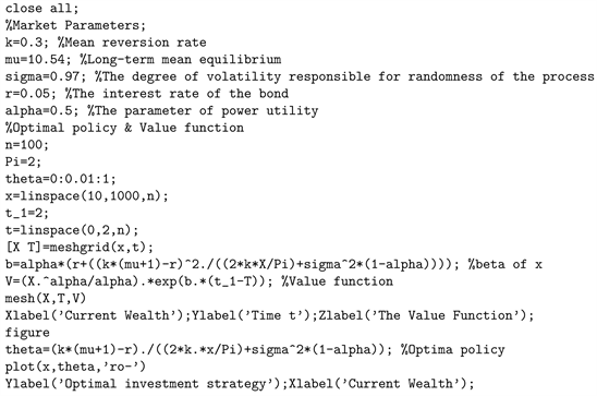
A.1. Codes for Numerical Simulation of Optimal Policy and Value Function for Power Utility Case

A.2. Codes for Numerical Simulation of Optimal Investment Strategy and Value Function for Exponential Utility Case

Conflicts of Interest

The authors declare no conflicts of interest.

References

[1]	Markowitz, H. (1952) Portfolio Selection. The Journal of Finance, 7, 77-91. https://doi.org/10.1111/j.1540-6261.1952.tb01525.x
[2]	Samuelson, P.A. (1969) Lifetime Portfolio Selection by Dynamic Stochastic Programming. The Review of Economics and Statistics, 51, 239-246. https://doi.org/10.2307/1926559
[3]	Merton, R.C. (1969) Lifetime Portfolio Selection under Uncertainty: The Continuous Time Case. Review of Economics and Statistics, 51, 247-257. https://doi.org/10.2307/1926560
[4]	Merton, R.C. (1971) Optimal Consumption and Portfolio Rules in a Continuous Time Model. Journal of Economic Theory, 3, 373-413. https://doi.org/10.1016/0022-0531(71)90038-X
[5]	Benth, F.E., Karlsen, K.H. and Reikvam, K. (2003) Merton’s Portfolio Optimization Problem in a Black-Scholes Market with Non-Gaussian Stochastic Volatility of Ornstein-Uhlenbeck Type. Mathematical Finance, 13, 215-244. https://doi.org/10.1111/1467-9965.00015
[6]	Zhai, J., Bai, M. and Wu, H. (2018) Mean-Risk-Skewness Models for Portfolio Optimization Based on Uncertain Measure. Optimization, 67, 701-714. https://doi.org/10.1080/02331934.2018.1426577
[7]	Chen, L., Peng, J., Zhang, B. and Rosyida, I. (2017) Diversified Models for Portfolio Selection Based on Uncertain Semivariance. International Journal of Systems Science, 48, 637-638. https://doi.org/10.1080/00207721.2016.1206985
[8]	Zhang, B., Peng, J. and Li, S. (2015) Uncertain Programming Models for Portfolio Selection with Uncertain Returns. International Journal of Systems Science, 46, 2510-2519. https://doi.org/10.1080/00207721.2013.871366
[9]	Merton, R.C. (1976) Continuous Time Portfolio Theory and the Pricing of Contingent Claims. MIT, Sloan School of Management, Working Paper Series, No. 881-76.
[10]	Luo, C. and Xi, Y. (2011) One Kind of Optimal Control Problem of Portfolio and Consumption Choice with Power Utility Function. International Journal of Pure and Applied Mathematics, 66, 331-337.
[11]	Khati, M.A. (2011) Portfolio Optimization in Discrete Time. AIMS, PGD Thesis.
[12]	Dmitrasinovic-Vidovic, G. and Ware, A. (2011) Optimal Portfolios of Mean-Reverting Instruments. SIAM Journal of Financial Mathematics, 2, 748-767. https://doi.org/10.1137/100787714
[13]	Dung, N.T. (2011) Fractional Geometric Mean-Reversion Processes. Journal of Mathematical Analysis and Applications, 380, 396-402. https://doi.org/10.1016/j.jmaa.2011.03.016
[14]	Emmer, S. and Klppelberg, C. (2004) Optimal Portfolios When Stock Prices Follow an Exponential Lévy Process. Finance and Statistics, 8, 17-44. https://doi.org/10.1007/s00780-003-0105-4
[15]	Koijen, R.S.J., Rodriguez, J.C. and Sbuelz, A. (2009) Momentum and Mean-Reversion in Strategic Asset Allocation. Journal of Management Science, 55, 1199-1213. https://doi.org/10.1287/mnsc.1090.1006
[16]	Munk, C., Sorensen, C. and Vinther, T.N. (2004) Dynamic Asset Allocation under Mean-Reverting Returns, Stochastic Interest Rates and Inflation Uncertainty: Are Popular Recommendations Consistent with Rational Behaviour? International Review of Economics and Finance, 13, 141-166. https://doi.org/10.1016/j.iref.2003.08.001
[17]	Poterba, J.M. and Summer, L.H. (1988) Mean-Reversion in Stock Prices: Evidence and Implications. Journal of Financial Economics, 22, 27-59. https://doi.org/10.1016/0304-405X(88)90021-9
[18]	Fleming, W.H. and Pang, T. (2004) A Stochastic Control Model of Investment, Production and Consumption. Quarterly of Applied Mathematics, 63, 71-87. https://doi.org/10.1090/S0033-569X-04-00941-1
[19]	Øksendal, B.K. (2003) Stochastic Differential Equations: An Introduction with Applications. 6th Edition, Springer-Verlag Publishers, Berlin.
[20]	Chaudhuri, K. and Wu, Y. (2004) Mean-Reversion in Stock Prices Evidence from Emerging Markets. Managerial Finance, 30, 22-37.
[21]	Pham, H. (2009) Continuous-Time Stochastic Control and Optimization with Financial Applications. Springer-Verlag, Berlin Heidelberg. https://doi.org/10.1007/978-3-540-89500-8
[22]	Ndounkeu, L.T. (2010) Stochastic Control: With Applications to Financial Mathematics. AIMS, PGD Thesis.
[23]	Karatzas, I. and Shreve, S.E. (1988) Brownian Motion and Stochastic Calculus. Springer-Verlag Inc., New York. https://doi.org/10.1007/978-1-4684-0302-2
[24]	SaB, J. (2007) Stochastic Control: With Applications to Financial Mathematics. Austrian Academy of Sciences, Vienna.
[25]	Yong, J. and Zhou, X.Y. (1999) Stochastic Controls, Hamiltonian Systems and HJB Equation. Springer-Verlag Inc., New York.