Methodology for Volumetric Measuring Transport of River Sand, in a Laboratory Channel with Mobile Bottom

Martín Mundo-Molina, Jose Luis Pérez-Díaz, Daniel Hernández-Cruz

Engineering Faculty, Chiapas State University, Tuxtla Gutiérrez Chiapas, Mexico.

DOI: 10.4236/eng.2018.1011053                

Abstract

Most public universities in Latin America and Mexico lack laboratories for measuring sediment transport or to do academic activities. The Research Center of the engineering faculty of Chiapas state university (UNACH by its acronym in Spanish) designed a portable prismatic channel for teaching and researching the sediment transportation in rivers. This paper presents the method to measure river sand transportation in a laboratory channel with a mobile bottom and presents the results of twenty-seven experiments done in the portable channel, using nine different slope inclinations and 27 flow and water speed values. The three main results are the following: 1) The construction of the channel with variable slopes, to experiment and measure sediment transportation. 2) A method developed for measuring the volume of sediment in a laboratory. 3) In a channel with a bottom slope of 0.071, a water flow of 2 l/s and a water speed of 1.77 m/s, the volume of transported sediment was 0.015 m³; in a channel with a bottom slope of 0.44, a water flow of 2 l/s and a water speed of 0.788 m/s, the volume of transported sediment was 0.006 m³; in a channel with the bottom slope of 0.024, a water flow of 2 l/s and a water speed of 0.62 m/s, the transported sediment was 0 m³.

Keywords

Volumetric Measurement of Sediment, Sediment Transport, Transportable Prismatic Channel, Measurement of Sediment in Laboratory

1. Introduction

Lack of economic resources for equipment and experimental research is one of the most critical problems in state universities of Latin America, especially in small towns. In order to collaborate in a solution about it the Research Center (RC) of the Faculty of Engineering of UNACH, Mexico, designed and built a prismatic hydraulic channel (PHC), with the goal to promote experimental research and improve teaching [1] [2] because, in the last 30 years, numerical and virtual models have replaced experimental research in Mexico. The PHC is a channel with a rectangular cross-section and mobile bottom which varies the channel’s slope, and it is 5 m long and 9 cm wide.

The physical models respond as part of the solution to the limitations of theoretical models [3] , especially when measuring sediment transport volume. The development of physical models and the construction of artificial channels in laboratories help solve many problems that theory alone is not capable of, either due to their mathematical complexity or deficit of computational tools and computing power [3] .

This work presents a method to estimate the volume of sand river sediment transported in a laboratory channel with a mobile bottom. It also introduces an empirical equation that results from 27 experiments done in the portable channel, using nine different slope inclinations and 27 water flow (Q) and water speed (v) values. The empirical equation quantifies the volume of transported sediments with precision. Of the twenty-seven channel slope values shown in Table 1, the first nine represent “torrent rivers” because their slopes are higher than 6%, while the other eighteen slopes between 1.8% and 6% represent “torrential rivers” [4] .

Recently, several investigations similar to the one published in this work have developed, below, the most relevant of them are the following: Analysis of bridge scours around piers [5] ; verification of geotubes behavior to protect bridge abutments from erosion [6] ; analysis of sediment transport in a hydraulic model of Madre de Dios river [7] ; experimental analysis of erosion pits formation underneath transverse barriers in a curved section of a river [8] and assessment of high risk erosion areas in small rivers, using a two-dimensional hydraulic model [9] . However, the most parallel research to this work in intention and method is the one presented by [10] who studied the sediment load in the Shat Al-Gharaf River in southern Irak and presents three empirical equations to calculate the discharge of sediments in selected sections of the river. In his work, [10] made different measurements to assess the number of suspended sediments; nonetheless, unlike [10] this work calculates the “total amount” of transported sediments through an empiric equation, which means the sum of suspended sediments plus sediments dragged through the bottom. Thus, this paper contributes with the process of the channel construction, the method to calculate and quantify the volume of transported sediment in the laboratory and the process to get the empirical equation for measuring the volume of sediment transported downstream.

2. Materials and Method

2.1. Materials

This investigation used a hydraulic channel with a rectangular cross-section of 9 cm wide, 5 meters long, and a variable slope (Photo 1). The walls and bottom of

Table 1. Water velocity, Froude number and volume of sediment transported.

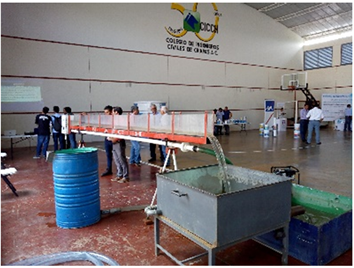
Photo 1. Hydraulic channel.

the PHC are acrylic. For support, the PHC has two tripods built with three steel pieces, 3 inches’ diameter each. The PHC is supplied with water through a 5 HP gasoline pump, connected to a small recirculation tank (SRT) that can store up to 600 liters of water [2] .

The SRT serves not only as a “reference model” to validate Q, but also as a deposit for water to circulate the water flow (Q) into the PHC (Photo 1). Figure 1 shows the calibration curve of the SRT.

The hydraulic channel has a gasoline pump of 5 HP with a 2-inch diameter of output, to drive water from the SRT to the PHC and to circulate the flow in a closed system.

The experiment used 1.5 m³ of coarse river sand collected from Suchiapa River (Photo 2), its diameter between 0.5 to 2 mm [4] [11] [12] . The Suchiapa River is located in Suchiapa municipality in Chiapas, México, at the following geographical coordinates: 16˚36'36''N and 93˚05'04''W.

The collected sediment is inorganic sand with an average diameter of about 2 mm. We moved the sediment to the soil mechanics laboratory of the UNACH, where its estimated weight was 1500 kg/m³.

2.2. Method

We spread a uniform layer of river sand, 6 cm thick, along the entire length of the bottom of the PHC (Photo 3 and Photo 4). According to Equation (1), the weight of the sand mass (W) was 40.5 kg.

$W=\gamma V$ (1)

where W is the weight of the soil mass in kg, $\gamma$ is the specific weight of the soil in kg/m³ and V is the volume in m³.

After placing the coarse river sand in the hydraulic channel, we circulated water, adjusting the bottom slope (So) and water speed until there was no sediment transport. This process was done in 4 hours, using a water flow of 2 l/s, that

Figure 1. Calibration curve of SRT.

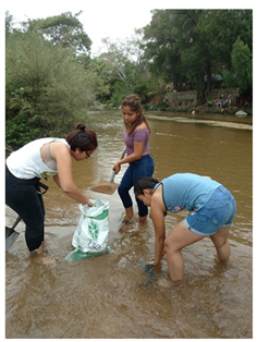
Photo 2. Students collecting river sand from Suchiapa River.

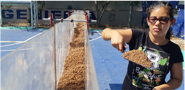
Photo 3. A student introducing coarse sand from the Suchiapa River in the hydraulic channel.

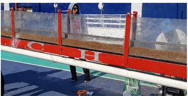
Photo 4. Water flow of 2 l/s and v = 0.5 m/s during 4 h.

circulated in the PHC with a velocity of 0.5 m/s, and a slope of S_o = 0. We measured the flow in l/s with the volumetric method, using the SRT and the next equation:

$Q=\frac{V}{t}$ (2)

where Q is the water flow (l/s), V is the volume (l) and t is the time (s).

The roughness coefficient of Manning was calculated with Equation (2) [13] :

$n=\frac{A_h{R}_h^{0.666}\sqrt{S_O}}{Q}$ (3)

where Q is the water flow in m³/s, A_h, is the hydraulic area in m², R_h is the hydraulic radius in m, and S_o is the slope of the PCH. The “n” obtained was 0.030. The design of the experiments include 27 slopes classified as “torrent slopes” and “torrential slopes”, each of these with three types of slope. For example, the torrent slopes shown in red in Figure 2 have three levels: high, medium and low. In the same way, torrential slopes shown in black and yellow were classified as high, medium and low, in order to simulate different conditions of sediment transport according its slope and Froude number.

For each slope in Figure 2, three types of water flow ranges were used: maximum, average and minimum. Figure 3 shows the three types of flow ranges of Q used in the twenty-seven experiments, which were 1.2 < Q < 3 l/s.

Thus, we collected the transported river sand with a cloth over a fine mesh, as shown in Photo 5, so we could measure its volume.

3. Results

The data collected from the 27 experiments was gathered in Table 1 which shows the main results:

As shown in Figure 4 and Table 1, if the water velocity decreases the hydraulic regime turns to a subcritical regime, and the sediment volume decreases, in this case are tending to zero.

There is a clear relationship between the reduction in the channel slope, the Froude number, flow velocity, and the sediment transported. Figure 5 shows the relationship between the volume of river sand transported (bottom and suspension sediment), water velocity and the empirical equation (see Equation (4)) for calculating the transported quantities of river sand in a laboratory channel with a mobile bottom.

$V=0.0007v^2-0.0511v+1.3863$ (4)

Figure 2. Bottom slopes of the PHC.

Figure 3. Ranges of maximum, average and minimum water flow used in the 27 experiments.

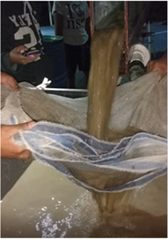
Photo 5. Collection of transported river sand.

where V is the volume in m³, and v is water velocity in m/s. Figure 6 shows the contrast between the results of the measured volume and the volume calculated with Equation (4), and Table 2 demonstrates the standard deviation, errors and statistical efficiency of the calculations and measurements.

4. Conclusion

The Research Centre of the Engineering Faculty of Chiapas State University designed and constructed a PHC in order to teach and do research on sediment transport. The channel has a rectangular cross-section and a variable slope, and its 5 m long and 9 cm wide. This work presents the PHC constructed, a method to measure the volume of sand river sediment transported in a laboratory channel, and an empirical equation that results from the 27 experiments done with

Figure 4. Water velocity of 27 experiments.

Figure 5. Relationship between volume of sediment transported and water velocity.

different slope values. The first nine slopes represent “torrent rivers” because its inclination is bigger than 6%, while the other eighteen slopes represent “torrential rivers”. We used coarse sand collected from the Suchiapa River, which was spread all along the bottom of the channel, in a uniform layer 6 cm thick. Its specific weight is 1500 kg/m³. We circulated water 27 times, each time with a different water flow and water velocity value, and the transported sand sediment was collected with a cloth over a mesh and quantified. According to the results, there is a clear relationship between the decrease in the channel slope, the Froude

Figure 6. Volume real and estimated.

Table 2. Standard deviation, errors and statistical efficiency.

number, water velocity and transported sediment. Based on the results, we developed an empirical equation to calculate the volume of transported river sand (bottom and suspended sediment) in a laboratory channel. This equation calculates with good precision the volume of sediment; it has a mean squared error of 0.00158 and an efficiency of statistical precision of 0.9353. Other results are: In a channel with a bottom slope of 0.071, a water flow of 2 l/s and a water velocity of 1.77 m/s, the volume of transported sediment was 0.015 m³; in a channel with a bottom slope of 0.44, a water flow of 2 l/s and a water velocity of 0.788 m/s, the volume of transported sediment was 0.006 m³; in a channel with the bottom slope of 0.024, a water flow of 2 l/s and a water velocity of 0.62 m/s, the transported sediment was 0 m³. For future investigations, it is necessary to study the total volume of suspended and transported sediment, but each one independently.

Conflicts of Interest

The authors declare no conflicts of interest.

References

[1]	Mundo-Molina, M. (2018) Volumetric Measuring of Sediments in a Transportable Prismatic Channel. 6th International Symposium on Sediment Management, San Cristóbal de las Casas, Chiapas.
[2]	Mundo, M.M. (2014) Diseño y construcción de un canal económico en el laboratorio de hidráulica de la Facultad de Ingeniería de la UNACH. Congreso Latinoamericano de hidraulica, Santiago de Chile.
[3]	Lopardo, R. (1995) La formación del ingeniero hidráulico para el siglo XXI. Revista Ingeniería del Agua, 2, 67-76. https://doi.org/10.4995/ia.1995.2688
[4]	Martín, J.P. (2003) Ingeniería de ríos. Ed. Alfaomega, México. D.F.
[5]	Ayala, L., Herrera, I., Cepeda, J. and Saldaña, A. (2018) Modelación numérica de la socavación local en pilas circulares con modelos lagrangianos. XXVIII Congreso Latinoamericano de Hidráulica, Buenos Aires, Argentina.
[6]	Spais, A., Reynares, M., Scacchi, G., Possi, M. and Schreider, M. (2018) El uso de geotubos como medida de protección de estribos de puentes. XXVIII Congreso Latinoamericano de Hidráulica, Buenos Aires, Argentina.
[7]	Cusipima, M., Kuroiwa, J. and Castro, L. (2018) Simulación numérica de la hidrodinámica y transporte de sedimentos en el modelo hidráulico del río Madre de Dios. XXVIII Congreso Latinoamericano de Hidráulica, Buenos Aires, Argentina.
[8]	Reyes, N., Kuroiwa, J. and Castro, L. (2018) Erosión aguas abajo de traviesas en tramos curvos: Resultados preliminares. XXVIII Congreso Latinoamericano de Hidráulica, Buenos Aires, Argentina.
[9]	Salinas, H., álvarez, A., Becerril, J. and García, J. (2018) Estimación de zonas de alto riesgo erosivo en ríos pequeños, utilizando un modelo hidráulico bidimensional. XXVIII Congreso Latinoamericano de Hidráulica, Buenos Aires, Argentina.
[10]	Maatooq, J., Omran, H. and Aliwe, H. (2016) Empirical Formula for Estimation the Sediment Load in Shat AL-Gharaf River. Basrah Journal for Engineering Sciences, 16, 38-41.
[11]	Maza, A.J.A. and García Flores, M. (1986) Distribuciones de los tamaños de los sedimentos del fondo en cauces naturales. Memorias del XII Congreso Latinoamericano de Hidráulica, 3, 104-109.
[12]	Maza, A.J. and García, F.M. (1996) Manual de Ingeniería de Ríos. Series del Instituto de Ingeniería. UNAM, México D.F.
[13]	Chow, V.T. (2004) Hidráulica de canales abiertos. Ed. Mc-Graw-Hill. Santa Fé de Bogotá, Colombia.