1. Introduction
The simplex method developed by Dantiz [2] has been widely used to solve many large-scale optimizing problems with linear constraints. Its practical performance has been good and researchers have found that the expected number of iterations exhibits polynomial complexity under certain conditions [3] [4] [5] [6] . However, Klee and Minty in 1972 gave a counter example showing that its worst case performance is
[7] . Their example is a deliberately constructed deformed cube that exploits a weakness of the original simplex pivot rule, which is sensitive to scaling [8] . It is found that, by using a different pivot rule, the Klee-Minty deformed cube can be solved in one iteration. But for all known pivot rules, one can construct a different deformed cube that requires exponential number of iterations to solve [9] [10] [11] . Recently, the interior point method [12] has been gaining popularity as an efficient and practical LP solver. However, it was also found that such method may also exhibit similar worse case performance by adding a large set of redundant inequalities to the Klee-Minty cube [13] .
Is it possible to develop a strongly polynomial algorithm to solve the linear programming problem, where the number of iterations is a polynomial function of only the number of constraints and the number of variables? The work by Barasz and Vempala shed some light in this aspect. Their AFFINE algorithm [14] takes only
iterations to solve a broad class of deformed products defined by Amenta and Ziegler [15] which includes the Klee-Minty cube and many of its variants.
In certain aspect, the Gravity Sliding algorithm [1] is similar to the AFFINE algorithm as it also passes through the interior of the feasible region. The main difference is in the calculation of the next descending vector. In the gravity falling approach, a gravity vector is first defined (see Section 3.1 for details). This is the principle gradient descending direction where other descending directions are derived from it. In each iteration, the algorithm first computes the descending direction, then it descends from this direction until it hits one or more facets that forms the boundary of the feasible region. In order not to penetrate the feasible region, the descending direction needs to be changed. The trajectory is likened a water droplet falling from the sky but is blocked by linear planar structures (e.g. the roof top structure of a building) and needs to slide along the structure. The core of gravity sliding algorithm is how to calculate the projection of the gravity vector g onto the intersection of a group of facets. This projection vector lies on the intersection of the facets and hence lies on the null space defined by these facets. Conventional approach is to compute the null space first and then find the projection of g onto this null space. An alternative approach is disclosed in [1] which operates directly from the subspace formed by the intersecting facets. This direct approach is more suitable to the Gravity Sliding algorithm. In this paper, we further present an efficient method to compute the gradient projections on complementary facets and also introduce the notion of selecting the steepest descend projection among a set of candidates. With these refinements, we rename the Gravity Sliding algorithm as the Sliding Gradient algorithm. We have implemented our algorithm and tested it on the Klee-Minty cube. We observe that it can solve the Klee-Minty deformed cube problem in only two iterations, irrespective of the dimension of the cube.
This paper is organized as follows: Section 2 gives an overview of the Cone-Cutting Theory [16] , which is the intuitive background of the Gravity Sliding algorithm. Section 3 discusses the Sliding Gradient algorithm in details. The pseudo-code of this algorithm is summarized in Section 4 and Section 5 gives a walk-through of this algorithm using the Klee-Minty as an example. This section also discusses the practical implementation issues. Finally, Section 6 discuss about future work.
2. Cone-Cutting Principle
The cone-cutting theory [16] offers a geometric interpretation of a set of inequality equations. Instead of considering the full set constraint equations in a LP problem, the cone-cutting theory enables us to consider a subset of equations, and how an additional constraint will shape the feasible region. The geometric insight forms the basis of our algorithm development.
2.1. Cone-Cutting Principle
In an m-dimension space
, a hyperplane
cuts
into two half spaces. Here
is the normal vector of the hyperplane and c is a constant. We denote the positive half space
the accepted zone of the hyperplane and the negative half space where
is rejected zone. Note that the normal vector
points to accepted zone area and we call the hyperplane with such orientation a facet
. When there are m facets in
and
are linear independent, this set of linear equations has a unique solution which is a point V in
. Geometrically,
form a cone and V is the vertex of the cone. We now give a formal definition of a cone, which is taken from [1] .
Definition 1. Given m hyperplanes in
, with rank
and intersection V,
is called a cone in
. The area
is called the accepted zone of C. The point V is the vertex and αj is the facet plane, or simply the facet of C.
A cone C also has m edge lines. They are formed by the intersection of (m − 1) facets. Hence, a cone can also be defined as follows.
Definition 2. Given m rays
shooting from a point V with rank
,
, the convex closure of m rays is called a cone in
.
is the edge,
the edge direction, and
the edge line of the cone C.
The two definitions are equivalent. Furthermore, P.Z. Wang [11] has observed that
and
are opposite to each other for
. Edge-line
is the intersection of all C-facets except
, while facet
is bounded by all C-edges except
. This is the duality between facets and edges. For
is called a pair of cone C.
It is obvious that
(for
) since
lies on
. Moreover, we have
(1)
2.2. Cone Cutting Algorithm
Consider a linear programming (LP) problem and its dual:
(Primary):
(2)
(Dual):
(3)
In the following, we focus on solving the dual LP problem. The standard simplex tableau can be obtained by appending an
identity matrix
which represents the slack variables as shown below:
We can construct a facet tableau whereby each column is a facet denoted as
, where
and
(4)
The facet tableau is depicted as follow. The last column
is not represented in this tableau.
When a cone
is intersected by another facet
, the ith edge of the cone is intersected by
at certain point
. We call
cuts the cone C and the cut points
can be obtained by the following equations:
(5)
The intersection is called real if
and fictitious if
. Cone cutting greatly alters the accepted zone, as can be seen from the simple 2-dimension example as shown in Figures 1(a)-(e). In 2-dimension, a facet
is a line. The normal vector
is perpendicular to this line and points to the accepted zone of this facet. Furthermore, a cone is formed by two non-parallel facets in 2-dimension. Figure 1(a) shows such a cone
. The accepted zone of the cone is the intersection of the two accepted zones of facets α1 and α2. This is represented by the shaded area A in Figure 1(a). In Figure 1(b), a new facet α3 intersects the cone at two cut points
and
. They are both real cut points. Since the arrow of normal vector
points to the same general direction of the cone, V lies in the rejected zone of α3 and we say α3 rejects V. Moreover, the accepted zone of α3 intersects with the accepted zone of the cone so that the overall accepted zone is reduced to the shaded area marked as B. In Figure 1(c),
points to the opposite direction. α3 accepts V and the overall
![]()
Figure 1. Accepted zone area of a cone and after it is cut by a facet.
accepted zone is confined to the area marked as C. As the dual feasible region 𝒟 of a LP problem must satisfy all the constraints, it must lie within area C. In Figure 1(d), α3 cuts the cone at two fictitious points. Since
points to the same direction of the cone, V is accepted by α3. However, the accepted zone of α3 covers that of the cone. As a result, α3 does not contribute to any reduction of the overall accepted zone area, and so it can be deleted for further consideration without affecting the LP solution. In Figure 1(e),
points to the opposite direction of the cone. The intersection between the accepted zone of α3 and that of the cone is an empty set. This means that the dual feasible region 𝒟 is empty and the LP is infeasible. This is actually one of the criteria that can be used for detecting infeasibility.
Based on this cone-cutting idea, P.Z. Wang [16] [17] have developed a cone-cutting algorithm to solve the dual LP problem. Each cone is a combination of m facets selected from (m + n) choices. Let D denotes the index set of facets of C, (i.e. if
, then
). The algorithm starts with an initial coordinate cone Co, then finds a facet
to replace one of the existing facet
thus forming a new cone. This process is repeated until an optimal point is found. The cone-cutting algorithm is summarized in Table 1 below.
This algorithm finds a facet that rejects V the least as the cutting facet in steps 2 and 3. This facet cuts the edges of the cone at m points. In step 4 and 5, the real cut point
that is closest to the vertex V is identified. This becomes the
vertex of a new cone. This new cone retains all the facets of the original cone except that the cutting facet replaces the facet corresponding to the edge I*. Yet the edge I* is retained but the rest of the edges must be recomputed as shown in step 6. Amazingly, P.Z. Wang shows that when
, this algorithm produces exactly the same result as the original simplex algorithm proposed by Dantz [2] . Hence, the cone-cutting theory offers a geometric interpretation of the simplex method. More significantly, it inspires the authors to explore new approach to tackle the LP problem.
3. Sliding Gradient Algorithm
Expanding on the cone-cutting theory, the Gravity Sliding Algorithm [1] was developed to find the optimal solution of the LP problem from a point within the feasible region 𝒟. Since then, several refinements have been made and they are presented in the following sections.
3.1. Determining the General Descending Direction
The feasible region 𝒟 is a convex polyhedron formed by constraints
, and the optimal feasible point is at one of its vertices. Let
be the set of feasible vertices. The dual LP problem (3) can then be stated as:
. As
is the inner-product of vertex
and b, the optimal vertex
is the vertex that yields the lowest inner-product value. Thus we can set the principle descending direction
to be the opposite of the b vector (i.e.
) and this is referred to as the gravity vector. The descending path then descends along this principle direction inside 𝒟 until it reaches the lowest point in 𝒟 viewed along the direction of b. This point is then the optimal vertex
.
3.2. Circumventing Blocking Facets
The basic principle of the new algorithm can be illustrated in Figure 2. Notice that in 2-dim, a facet is a line. In this figure, these facets (lines) form a closed polyhedron which is the dual feasible region 𝒟. Here the initial point P0 is inside 𝒟. From P0, it attempts to descend along the
direction. It can go as far as P1 which is the point of intersection between the ray
and the facet α1. In essence, α1 is blocking this ray and hence it is called the blocking facet relative to this ray. In order not to penetrate 𝒟, the descending direction needs to change from g0 to g1 at P1, and slides along g1 until it hits the other blocking facet α2 at P2. Then it needs to change course again and slides along the direction g2 until it hits P3. In this figure, P3 is the lowest point in this dual feasible region 𝒟 and hence it is the optimal point
.
It can be observed from Figure 2 that g1 is the projection of g0 onto α1 and g2 is the projection of g0 onto α2. Thus from P1, the descending path slides along α1 to reach P2 and then slides along α2 to reach P3. Hence we call this algorithm Sliding Gradient Algorithm. The basic idea is to compute the new descending direction to circumvent the blocking facets, and advance to find the next one until it reaches the bottom vertex viewed along the direction of b.
Let
denotes the set of blocking facets at the tth iteration. From an initial point P0 and a gradient descend vector g0, the algorithm iteratively performs the following steps:
1) compute a gradient direction gt based on
. In this example, the initial set
![]()
Figure 2. Sliding gradient illustration.
of blocking facets
is empty and
.
2) move
to
along
where
is a point at the first blocking facet.
3) Incorporate the newly encountered blocking facet to
to form
.
4) go back to step 1.
The algorithm stops when it cannot find any direction to descend in step (1). This is discussed in details in Section 3.6 where a formal stopping criterion is given.
3.3. Minimum Requirements for the Gradient Direction gt
For the first step, the gradient descend vector
needs to satisfy the following requirements.
Proposition 1.
must satisfy
so that the dual objective function
will be non-increasing when y move from
to
along the direction of
.
Proof. Since
,
aligns to the principle direction of
. As
,
moves along the principle direction of
when
.
Since
,
when
. END
This means that if
, then
is “lower than”
when viewed along the b direction.
Proposition 2. If
,
must satisfy
for all
to ensure that
remains dual feasible (i.e.
).
Proof. If for some j,
, this means that
is in the opposite direction of the normal vector of facet
so a ray
will eventually penetrate this facet for certain positive value of t. This means that Q will be rejected by
and hence Q is no longer a dual feasible point. END
3.4. Maximum Descend in Each Iteration
To ensure that
, we need to make sure that it won’t advance too far. The following proposition stipulates the requirement.
Proposition 3. Assuming that 𝒟 is non-empty and
. If
satisfies Propositions 1 and 2; and not all
for
, then
provided that the next point
is determined according to (6) below:
(6)
where
.
Proof. The equation for a line passing through P along the direction g is
. If this line is not parallel to the plane (i.e.
), it will intersect a facet
at a point Q according to the following equation:
. (7)
We call t the displacement from P to Q. So
is the displacement from
to αj. The condition tj > 0 ensures that
moves along the direction
but not the opposite direction.
is the smallest of all the displacements thus
is the first blocking facet that is closest to
.
To show that
, we need to show
for
. Note that
.
Since
,
for
, so we need to show that
for
.
The displacements
can be split into two groups. For those displacements where
,
so
, where
is a positive constant. Since
.
since
&
.
For those displacements where
, we have that
is the minimum of all
in this group. Let
be the ratio between
and
. Obviously,
So
. END
If
,
is parallel to
. Unless all facets are parallel to
, Proposition 3 can still find the next descend point
. If all facets are parallel to
, this means that facets are linearly dependent with each other. The LP problem is not well formulated.
3.5. Gradient Projection
We now show that the projection of
onto the set of blocking facets
satisfies the requirements of Proposition 1 and 2. Before we do so, we discuss the projection operations in subspace first.
3.5.1. Projection in Subspaces
Projection is a basic concept defined in vector space. Since we are only interested in the gradient descend direction of
but not the actual location of the projection, we can ignore the constant c in the hyperplane
. In other words, we focus on the subspace
spanned by
and its null space
rather than the affine space spanned by the hyperplanes.
Let Y be the vector space in
,
and its corresponding null space is
. Extending to k hyperplanes, we have
and the null space is
. It can be shown that
. Since
and
are the orthogonal decomposition of the whole space Y, a vector g in
can be decomposed into two components: the projection of g onto
and the projection of g onto
. We use the notation
and
to denote them and they are called direct projection and null projection respectively.
The following definition and theorem were first presented in [1] and is repeated here for completeness.
Let the set of all subspaces of
be 𝒩, and let 𝒪 stand for 0-dim subspace, we now give an axiomatic definition of projection.
Definition 3. The projection defined on a vector space Y is a mapping
where * is a vector in Y, # is a subspace X in 𝒩 satisfying that
(N.1) (Reflectivity).
For any
;
(N.2) (Orthogonal additivity).
For any
and subspaces
, if X and Z are orthogonal to each other, then
, where
is the direct sum of X and Z.
(N.3) (Transitivity).
For any
and subspaces
,
,
(N.4) (Attribution).
For any
and subspace
,
, and especially,
(N.5) For any
and subspace
,
.
A convention approach to find
is to compute it directly from the null space
. We now show another approach that is more suitable to our overall algorithm.
Theorem 1. For any
, we have
(8)
where
are an orthonormal basis of subspace
.
Proof. Since
and
are the orthonormal decomposition of Y, according to (N.2) and (N.1) we have
.
According to (N.2) and (N.4), the first term becomes
.
Hence (8) is true. END
The following theorem shows that the projection of
onto the set of all blocking facets σt always satisfies Propositions 1 and 2. First, let us simplify the notation and use σ to represent σt in the following section and
to stand for
where
is the number of elements in σ.
Theorem 2.
and
for all
.
Proof. Since
lies on the intersection of
, it lies on each facet
for
. Thus
is perpendicular to the normal vector of
(i.e.
). So it satisfies Proposition 2.
According to (N.5),
. So it satisfies proposition 1 too. END
As such,
, the projection of
onto all the blocking facets, can be adopted as the next gradient descend vector
. Hence,
, the projection of
onto all the blocking facets, can be adopted as the next gradient descend vector
.
3.5.2. Selecting the Sliding Gradient
In this section, we explore other projection vectors which also satisfy Propositions 1 and 2. Let the jth complement blocking set
be the blocking set σ excluding the jth element; i.e.
. We examine the
projection
for
. Obviously,
according to (N.5) as
is a projection of
. So if
for all
,
it satisfies Proposition 2 and hence is a candidate for consideration. For all the candidates, including
, which satisfy this proposition, we can compute the inner product of each candidate with the initial gradient descend vector
, (i.e.
) and select the maximum. This inner product is a measure of how close or similar a candidate is to
so taking the maximum means getting the steepest descend gradient. Notice that if a particular
is selected as the next gradient descending vector, the corresponding
is no longer a blocking facet in computing
. Thus
needs to be removed from
to form the set of effective blocking facets
. The set of blocking facets for the next iteration
is
plus the newly encountered blocking facet. In summary, the next gradient descend vector
is:
(9)
where
with
and
.
The effective blocking set
is
. (10)
At first, this seems to increase the computation load substantially. However, we now show that once
is computed,
can be obtained efficiently.
3.5.3. Computing the Gradient Projection Vectors
This session discusses a method of computing
and
for any vector g. According to (8),
. The orthonormal basis
can be obtained from the Gram Schmidt procedure as follows:
(11)
(12)
Let us introduce the notation
to denote the projection of vector a onto vector b. We have
, then
as
. Likewise,
. (13)
Thus from (8),
. (14)
After evaluating
, we can find
backward from
to 1. Firstly,
. (15)
Likewise, it can be shown that
. (16)
The first summation is projections of g onto existing orthonormal basis
. Each term in this summation has already been computed before and hence is readily available. However, the second summation is projections on new basis
. Each of these basis must be re-computed as the facet
is skipped in
. Let
(17)
. (18)
Then we can obtain
recursively from
by:
. (19)
To compute
, some of the intermediate results in obtaining the orthonormal basis can also be reused.
Let
for all
and
for
, then we have
. (20)
The intermediate terms
can be reused in computing
as follows:
. (21)
By using these intermediate results, the computation load can be reduced substantially.
3.6. Termination Criterion
When a new blocking facet is encountered, it will be added to the existing set of blocking facets. Hence both
and
will typically grow in each iteration unless one of the
is selected as
. In this case,
is deleted from
according to (10). The following theorem, which was first presented in [1] shows that when
, the algorithm can stop.
Theorem 3 (Stopping criterion) Assuming that the dual feasible region 𝒟 is non-empty, let
and is descending along the initial direction
; let
be the number of effective blocking facets in
at the tth iteration. If
and the rank
, then
is a lowest point in the dual feasible region 𝒟.
Proof. If
and the rank
, then the m facets in
form a cone C with vertex
. Since the rank is m, its corresponding null space contains only the zero vector. So
.
As mentioned about the facet/edge duality in Section 2, for
, edge-line
is the intersection of all C-facets except
. That means
. Since an edge-line is a 1-dimensional line, the projection of a vector
onto
equals to
and hence
. Since
are projections of
, according to (N.5),
.
Since
, it means that
does not satisfy Proposition 2 for all
. Otherwise, one of the
would have been selected as the next gradient descend vector and, according to (10), it would be deleted from
and hence
would be less than m. This means that at least one of
has a value
. However, for all
,
is in the null space of
so
. This leaves
. If
, then
. This contradicts to the fact that
in (1). Therefore,
. Since
,
. Note that
means that edge
is in opposite direction of
. As this is true for all edges, there is no path for
to descend further from this vertex. It is obvious that the vertex V is the lowest point of C when viewed in the b direction.
Since
is dual feasible, and V is a vertex of 𝒟. Cone C coincides with the dual feasible region 𝒟 in a neighborhood N of V, it is obvious that
is the lowest point of 𝒟 when viewed in the b direction. END
In essence, when the optimal vertex
is reached, all the edges of the cone will be in opposite direction of the gradient vector
. There is no path to descend further so the algorithm terminates.
4. The Pseudo Code of the Sliding Gradient Algorithm
The entire algorithm is summarized as follows in Table 2.
Step 0 is the initialization step that sets up the tableau and the starting point P. Step 2 is to find a set of initial blocking facets σ in preparation of step 4. In the inner loop, Step 4 calls the Gradient Select routine. It computes
and
in view of σ using Equations (11) to (21) and select the best gradient vector g according to (9). This routine not only returns g but also the effective blocking facets
and
for subsequent use. Theorem 3 states that when the size of
reaches m, the optimal point is reached. So when it does, step 5 returns the optimal point and the optimal value to the calling routine. Step 6 is to find the closest blocking facet according to (6). Because P lies on every facets of σ,
for
. Hence, we only need to compute those
where
. The newly found blocking facet is then included in σ in step 7 and the
![]()
Table 2. The sliding gradient algorithm.
inner loop is repeated until the optimal vertex is found.
5. Implementation and Experimental Results
5.1. Experiment on the Klee-Minty Problem
1Other derivations of the Klee-Minty formulas have also been tested and the same results are obtained.
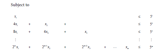
We use the Klee-Minty example presented in [18] 1 to walk through the algorithm in this section. An example of the Klee-Minty Polytope example is shown below:
.
For the standard simplex method, it needs to visit all
vertices to find the optimal solution. Here we show that, with a specific choice of initial point
, the Sliding Gradient algorithm can find the optimal solution in two iterations―no matter what the dimension m is.
To apply the Sliding Gradient algorithm, we first construct the tableau. For an example with
, the simplex tableau is:
The b vector is
. After adding the slack variables, the facet tableau becomes:
Firstly, notice that
and
have the same normal vector (i.e.
) so we can ignore
for further consideration. This is true for all value of m.
If we choose
, where M is a positive number (e.g.
), It can be shown that
is inside the dual feasible region. The initial gradient descend vector is:
.
With
and
as initial conditions, the algorithm proceeds to find the first blocking facet using (6). The displacements
for each facet can be found by:
.
With
and
as initial conditions, the algorithm proceeds to find the first blocking facet using (6). The displacements
for each facet can be found by:
. (22)
We now show that the minimum of all displacements is
.
First of all, at = m,
,
and
, so
.
For
,
, so
.
For
,
, and the elements of
are:
.
The 2nd term of Equation (22) can be re-written as:
The inner product of the denominator is:
Since all the elements in the b vector and the
are positive, the summation is a positive number. Thus
Since the value of the denominator is bigger than
, we have
So
.
Hence
is the smallest displacement. For the case of
, their values are shown in the first row (first iteration) of the following Table 3.
Thus
is the closest blocking facet. Hence,
. For the next iteration,
.
The gradient vector
is
projects onto
. Because
is already an orthonormal vector, we have according to (8)
.
In other words,
is the same as
except that the last element is zeroed out. Using
and
, the algorithm proceeds to the next iteration and evaluates the displacements
again. For
to
, since
and
is a unit vector with only one non-zero entry at the jth element,
.
Thus the displacements
to
have the same value of
.
For
, we have:
.
As mentioned before,
is the same as
except that the last element is zero, we can express
in terms of
as follows:
.
The numerator then becomes:
.
Since
,
and
, substituting these values to the above equation, the numerator becomes
.
Thus
.
![]()
Table 3. Displacement values
in each iterations for
.
Notice that all elements in
are negative but all of
are positive. So the inner product
is a negative number. As a result, the last term inside the bracket is a positive number which makes the whole value inside the bracket bigger than one and hence
for
. Moreover,
is zero as
lies on
. The actual displacement values for the case of
are shown in the second row of Table 3.
Since
to
have the same lowest displacement value, all of them are blocking facets so
. Also,
.
Now
, so
has reached a vertex of a cone. According to Theorem 3, the algorithm stops. The optimal value is
, which is the last element of the b vector.
Thus with a specific choice of the initial point
, the Sliding Gradient algorithm can solve the Klee-Minsty LP problem in two iterations, and it is independent of m.
5.2. Issues in Algorithm Implementation
The Sliding Gradient Algorithm has been implemented in MATLAB and tested on the Klee-Minty problems and also self-generated LP problems with random coefficients. As a real number can only be represented in finite precision in digital computer, care must be taken to deal with the round-off issue. For example, when a point P lies on a plane
, the value
should be exactly zero. But in actual implementation, it may be a very small positive or negative number. Hence in step 2 of the aforementioned algorithm, we need to set a threshold δ so that if
, we regard that point P is laid on the plane. Likewise for the Klee-Minty problem, this algorithm relies on the fact that in the second iteration, the displacement values
for
to
should be the same and they should all be smaller than the values of
for
to
. Due to round-off errors, we need to set a tolerant level to treat the first group to be equal and yet if this tolerant level is set too high, then it cannot exclude members of the second group. The issue is more acute as m increases. It will require higher and higher precision in setting the tolerant level to distinguish these two groups.
6. Conclusions and Future Work
We have presented a new approach to tackle the linear programming problem in this paper. It is based on the gradient descend principle. For any initial point inside the feasible region, it will pass through the interior of the feasible region to reach the optimal vertex. This is made possible by projecting the gravity vector to a set of blocking facets and using that as descending vector in each iteration. In fact, the descending trajectory is a sequence of line segments that hug either a single blocking facet or the intersections of them, and each line segment is advancing towards the optimal point. It should be noted that there is no parameters (such as step-size, ..., etc.) to tune in this algorithm although one needs to take care of numerical round-off issue in actual implementation.
This work opens up many areas of future research. On the one hand, we are extending this algorithm so that it can relax the constraint of starting from a point inside the feasible region. Promising development has been achieved in this area though more thorough testing on obscure cases need to be carried out.
On the theoretical front, we are encouraged that, from the algorithm walk-through on the Klee-Minty example, this algorithm exhibits strongly polynomial complexity characteristics. Its complexity does not appear to depend on the bit sizes of the LP coefficients. However, more rigorous proof is needed and we are working towards this goal.
Acknowledgements
The authors wish to thank all his friends for their valuable critics and comments on the research. Special thanks are given to Prof. Yong Shi, Prof. Sizong Guo for their supports. This study is partially supported by the grants (Grant Nos. 61350003, 70621001, 70531040, 90818025) from the Natural Science Foundation of China, and grant (Grant No. L2014133) from Department of Education of Liaoning Province.