Development and Application of a Modified Genetic Algorithm for Estimating Parameters in GMA Models ()
1. Introduction
Although in many instances the standard mathematical approach to the modelling of biochemical systems has been the so called Michaelis-Menten formalism [1] -[3] , there is a growing amount of evidences on the efficacy and advantages of the Power-Law alternative mathematical representation [4] -[7] . Within this formalism, several choices are available for the formulation of biochemical pathways, and the most successful one is Generalized Mass Action (GMA) system [5] . The basic concepts of the power-law formalism have been described many times [5] [8] .
The Generalized Mass Action representation [5] has the following structure:
 (1)
(1)
where Xi represents any of the n dependent variables of the model (e.g., intermediary metabolites, enzyme activity, substrates and biomass concentrations, etc.). Here, as shown above, the rate of each sub-process j is expanded as a product of a rate constant (γj) and the n + m system variables Xk, which are influencing Xi through the so-called kinetic orders (gjk), while cij gives the stoichiometric coefficient of the considered element Xi in the reaction j. The independent variables are those that are fixed or controlled by the experimenter, and they could differ under different situations. Power-law models, as the one shown above, allow capturing complex dynamics, e.g. saturation behaviour, inhibition or cooperativity [5] [7] .
Parameter estimation is a recurrent issue in the model building process. It deals with the finding of the numerical values characterizing the mathematical representation of a given system from experimental data [9] . A key feature of the experimental measurements is that they must come from variables representing their main features both at a given particular time as well as along its evolution over time [10] . When the model is defined in terms of algebraic equations dependent on the system variables and the experimental data are time series, obtaining the model parameters becomes a regression problem [11] . In this context calibration is a global optimization problem [5] [12] in which it is necessary to minimize the distance between the experimental data and those generated by the model. It is global because it does not suffice to find a minimum, but the smallest of them all. The distance is the magnitude to be used as cost or objective function in an optimization problem [10] . This function would depend on the experimental data and on the parameter values. When there are several experimental curves of the same system (as it is usually the case) it can be more than only one cost function, thus the estimation process becoming a multi-objective global optimization problem.
Although there are many optimization algorithms, there are usually not global ones and very few multi- objective global optimizations [10] [13] but all of them belong to one of two main classes: deterministic or heuristic. The first ones use information directly from the p dimensions data surface, (p being the number of parameters) or try to modify it as gradients, giving it a global convexity so that it would be possible to use local methods in order to reach the optimum. Heuristic methods try to find a fast and acceptable solution although they cannot guarantee the solution are the best possible. Genetic algorithms belong to this type, being a special type of evolutionary algorithms [14] [15] . These algorithms, which are classified as global optimizers, use techniques inspired by evolutionary biology.
Genetic Algorithms mimic the evolutionary dynamics of a population [16] . In its classical presentation the population consists on a set of individuals, each one containing a genotype, the coded characteristics of the represented solution, and a phenotype, the value of the objective function [14] . Depending on the type of problem the initial population can be randomly generated or according to a predetermined procedure. In each generation individuals are selected to create new elements of the population by combining their genotypes or, alternatively, to belong to the next generation according to its phenotype. In this way, in each generation new individuals compete for survival with those who are considered the best of the previous generation [17] . The process ends when the goal is reached or the solution is close enough to the required one.
In this work we will introduce a modified version of the simple genetic algorithm and will show the results of its application to two GMA models to illustrate its utility and potentialities as a method for parameter estimation in complex model systems of biological significance.
2. The Modified Genetic Algorithm
The structure of the proposed Modified Genetic Algorithm (MGA) is shown in Figure 1. The proposed method

Figure 1. Flow chart of the modified genetic algorithm.
has several distinctive features and is structured according to three main traits: the process of selection, the use of a Hill Climbing local method, and the fact that the total population size is selectable although remaining constant between generations.
2.1. Objective Function
The objective function for parameter estimation using experimental data corresponds to the squared distance between these points and those generated by introducing the estimated parameters in the model, as described in Equation (2)
 (2)
(2)
where  represents the i-th experimental data of the j-th curve;
  stands for the value generated by the model for a given set of parameters θ;
  corresponds to the value of the experimental error for that point; np is the total number of points of each curve and nc the total number of curves. As can be seen the multiobjective problem has been transformed into a single-objective one by taking as objective function the sum of all the objective functions [18] .
2.2. Generation of the Initial Population
The very first step in developing the procedure is the selection of the elements of the initial population. They are randomly generated from predefined parameter limits while the associated objective function is evaluated. In this way the MGA allows the definition and application of a cut-off criteria based on the function cost, so that all initial elements have a preselected good fit to the experimental data. This feature helps to increase the speed of convergence, but at the expense of investing some extra runtime at the start-up.
2.3. Sorting the Population
In each step before Selection (see below) the population is sorted in a list. To do that all solutions are named by an index which indicates the position of the solution on the list. The position on the list depends on the value of the objective function of the solution. In this way the lesser value of the objective function of the element, the smaller the index of the element in the population.
2.4. Temporal Population
A temporal population is created using the initial population. First, it is defined the population size (before the algorithm is launched). After that, the individuals of this temporal population are obtained in pairs by crossing two random individuals of the initial population (see below), these two new individuals are added to the temporal population and the process continues until the defined size is reached.
2.5. Coding
Before proceeding to the mutation and crossing of two given individuals, their parameters are converted to binary code and placed in order to form a chain. Later, after the next step of mutation and crossover (see below) the binary chain will be recoded in real values.
2.6. Mutation and Crossover
After being selected and encoded into binary strings, the two individuals become subject of mutation and crossover operators as defined by Holland [14] . The crossing process implies the selection of a number of points that serve to create a new pair of individuals containing a mixture of binary strings of the initial, parental, individuals. In our MGA it is possible to define a range for the number of crossing points, while the points themselves are chosen randomly. The mutation, in turn, modifies some bits of the new individuals so generated; the MGA is able to control the probability of any bit string to be modified.
2.7. Parameter Control
An independent control is performed on each generating process. This is done either at the mutation and crossing step or at the Hill-Climbing local search (see below). In this way the algorithm is able to check whether the values of the parameters remain within the initially defined ranks. In the case that no individual fulfils the prescribed criteria, a high value of the objective function is assigned, forcing thus to be released in subsequent generations.
2.8. Selection
The MGA performs three selection processes on the total population. The first one, just at the beginning of each iteration, selects those individuals on which the mutation and crossover operators will be applied. The second one is aimed to select those individuals that will be the subject of a Hill-Climbing local searching optimization (see below). Finally, a selection of the individuals that will form the population of the next generation is carried out. The selection of each individual picked in the former processes is fulfilled by using the following
 (3)
(3)
when Rand is a random number evenly distributed between zero and one, Int is the integer operator, size is the population size and b is a control constant. When b equals 1 the choice is made uniformly, so that it is equally likely to choose an individual with a better or worse value of the objective function. If b is greater than 1, the individuals with smaller objective function are more probably selected. For example, with b = 2, about a 50% of the selected would belong to the first quarter of the sorted population. It is thus clear that the value of b is critical, since a high value will cause a rapid convergence towards local optimum with a significant loss of population diversity, but a low b will increase computational costs. Finally, it should be noted that while the first and second selection processes may select the same individual several times, the third one cannot select twice the same individual, so duplicates are avoided.
2.9. Hill-Climbing Local Search
Every few generations (a controllable value) a number of individuals of the total population are chosen as starting points of a local search. In each of these starting points, parameters are changed in a small and random amount and the new objective function evaluated. If the new value is lower than it was initially, the new set of parameters is adopted, otherwise they are kept at the original ones. Both the number of times to repeat the process as well as how much the original parameters can be changed are controllable values.
2.10. Stopping Criterion
The algorithm can come to an end in two cases. The first one is when it reaches a cost function value smaller than a previously defined one. The second one occurs when a certain number of generations is reached. It is also possible to set up a combination of both. In the following case studies it will be shown how this criterion, in which we will target the sum of the objective functions, is applied to multi-experiment adjustments.
The algorithm has been programmed on MathWorks Matlab 7.5 and executed on a PC PIV 2.0 Ghz, 1GB RAM.
3. Results
3.1. Case Study 1: Branched Pathway
The branched pathway system shown in Figure 2 Error: No se encuentra la fuente de referencia is a theoretical, general case study used for system analysis and testing purposes [10] . It has four variables, six flows and two control loops.
The corresponding GMA model [5] is shown in Equations (4). The model has thirteen parameters to be estimated: six reaction rates values (γ1 to γ6) and seven kinetic orders (g1 to g7).
 (4)
(4)
For the purpose of evaluation and comparison with other estimation algorithms, results obtained with MGA were checked against those obtained by using other two different parameter estimation algorithms provided within the Optimization Toolbox package of MathWorks Matlab 7.5, namely the Simulated Annealing [19] and the Simple Genetic Algorithm. For each of the methods a constant population of 500 individuals was used and
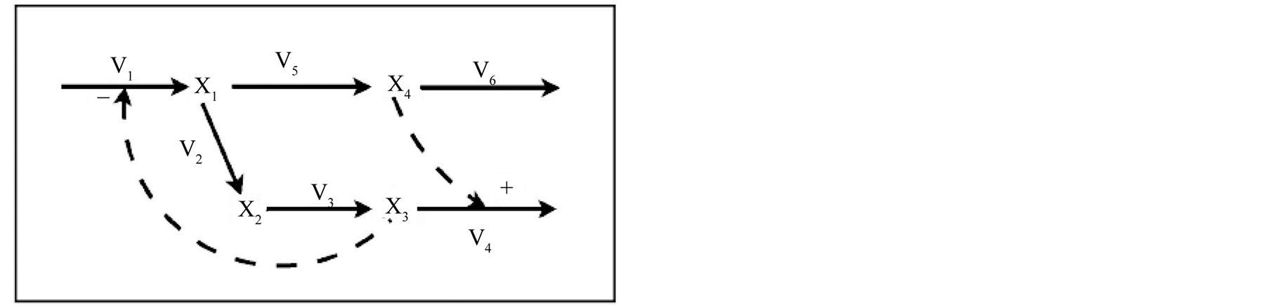
Figure 2. Branched pathway model. Arrows represent fluxes while dashed lines regulatory interactions. X1 to X4 represent metabolic intermediates. Plus and minus signs indicate activating and inhibiting interactions respectively.
the process repeated 50 times. In the case of MGA, the Hill-Climbing routine was inserted every 10 generations with b equal to 1.2 for each selection process. The computation time with the SGA and the MGA were 15% and 20% slower than SA, respectively.
In this study, provided with a set of actual parameters values, we were able to generate a set of experimental data. This was done from a given initial, non-steady state condition, from which a numerical solution was obtained and subsequently discretized into a series of evenly distributed points along the time interval 0 to 5. We then made use of the generated data to obtain the initial set of parameters values. Moreover, in order to test method reliability, we tested the method predictions in presence and absence of noise. In the first case this was done by adding some random variable noise to the very same system definition (depending on the value of each point) associated to the simulated experimental data, thus mimicking in this way the real situation. Table 1 shows the estimated parameter sets obtained from each assayed method at the two noise conditions. It can be seen that all methods yield essentially the same results, but by some accounts the MGA gives the best estimates.
Figure 3 shows the curves obtained from each estimated parameter set. In panels (a), (c) and (e) results obtained
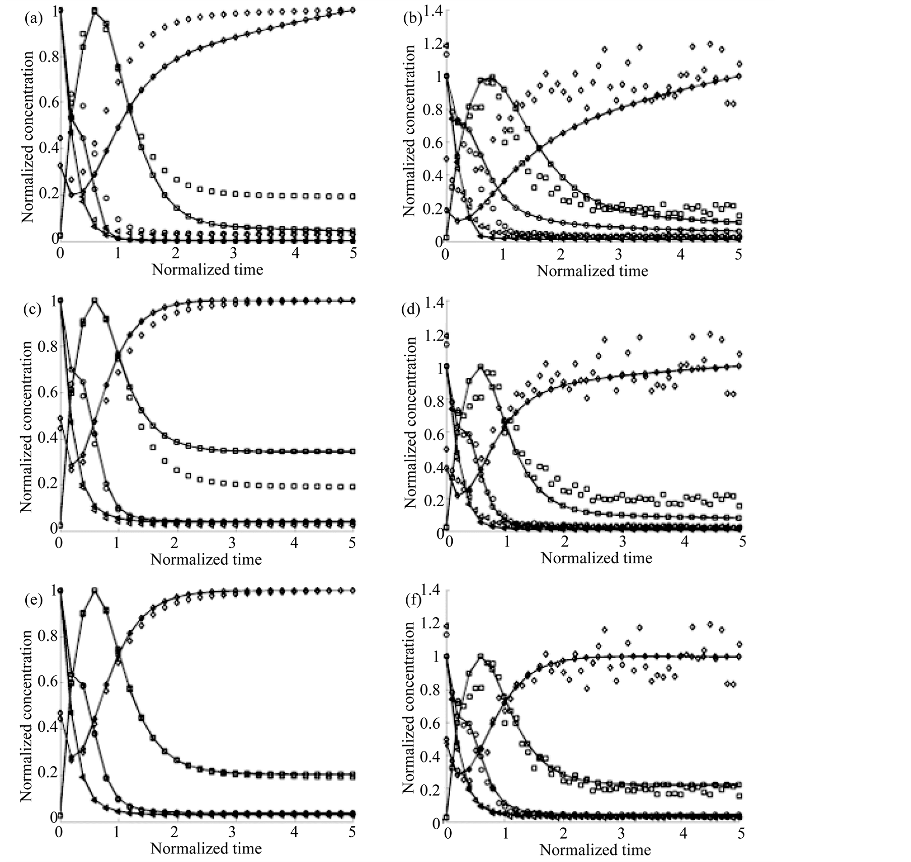
Figure 3. Estimation curves for the Branched Pathway Model. Continuous lines represent the results of adjustment while dotted ones represent the numerical integration of the original model. X1: ○; X2: □; X3: ◊ and X1: ∆. (a) and (b) show the results obtained by using Simulated Annealing without and with noise, respectively; (c) and (d) correspond to the Simple Genetic Algorithm without and with noise, respectively and (e) and (f) are the results using the MGA, without and with noise respectively.

Table 1. Estimated parameter values for the Branched Pathway Model with and without noise data. Actual values are shown together with deviations of estimated values by using three methods: SA: Simulated Annealing; SGA: Simple Genetic Algorithm; MGA: Modified Genetic Algorithm. AV stands for the actual parameter values.
in absence of noise are shown. These results correspond to a 2000 generations execution, when the selected ranges for the parameters were [0, M] for the positive and [‒M, 0] for negative; being M twice the absolute value of each of the original parameters. When noise was present, we obtained the results shown in panels (b), (d) and (f).
3.2. Case Study 2: The JAK2-STAT5 Signaling Pathway
In a previous work [20] a combination of qualitative biological knowledge and experimental data was used to establish the structure of a mathematical, power law model, of the amplification and responsiveness of the JAK2/STAT5 pathway. The proposed MGA algorithm was used to determine the values of its parameters. Figure 4 illustrates the structure and the proposed model variables [20] . The model includes the recruitment of erythropoietin receptor (EpoR) to the plasma membrane; the activation by Epo and the deactivation of the EpoR/JAK2 complex as well as the phosphorylation, dimerization and nucleocytoplasmic shuttling of STAT5. It is assumed that the EpoR and the JAK2 kinase form a stable complex, EpoR/JAK2. Two possible states for the EpoR/JAK2 complex are considered: Epo not bound to EpoR/JAK2 complex, EJ, and Epo bound to EpoR/JAK2 complex and therefore the EpoR/JAK2 complex activated, pEpJ. The dephosphorylation and deactivation processes of the complex by phosphatases is considered. The model includes terms describing the recruitment of new EpoR/JAK2 complexes to the plasma membrane and the internalization and subsequent degradation of non-activated EpoR/JAK2 complexes. Three possible states have been considered for STAT5 in the model and since the dimerization of activated STAT5 is a fast process, the model assumes that the protein dimerizes immediately after activation; the variable describing monomeric STAT5 being neglected. The model describes the fraction of STAT5 inside the nucleus with a single state variable. The concentration of erythropoietin in the extracellular medium (Epo) is considered the input signal of the system. The resulting model has five dependent variables and one input variable (Equations (5)).
 (5)
(5)
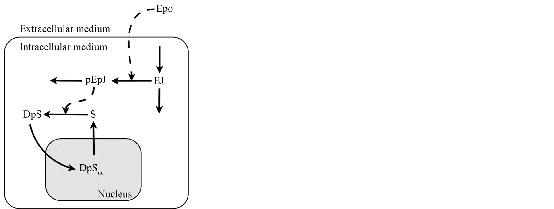
Figure 4. Structure of the JAK2-STAT5 pathway model. Epo: concentration of Epo in the extracellular medium; EJ: fraction of non-activated EpoR/JAK2 complex; pEpJ: fraction of activated EpoR/JAK2 complex; S: fraction of non-activated and non-dimerised STAT5 in the cytosol; DpS: fraction of activated and dimerized STAT5 in the cytosol; DpSnc: fraction of activated and dimerized STAT5 inside the nucleus.
In this study, parameters were computed for biologically feasible intervals in the parameter space using the MGA algorithm. The parameter values for the chosen model are summarized in Table2
The model trajectories obtained with the chosen solution are depicted in Figure 5.
4. Discussion
The analysis of the results obtained from the application of the MGA to the two case studies presented allows a preliminary evaluation of the potentialities and shortcomings of the proposed algorithm.
Results obtained from the Case 1 study indicate that the MGA has significant advantages when compared with the SGA and the SA algorithms. As it can be seen in Figure 3 the MGA gives far better fitting that the others with the same number of iterations both in the presence (Figure 3(b), Figure 3(d) and Figure 3(f)) and absence of noise (Figure 3(a), Figure 3(c) and Figure 3(e)). Table 1 shows also that the MGA algorithm gives more accurate estimations of the original model parameters both in presence and absence of noise conditions. The mean relative error between the actual parameter values and the estimated in the case of MGA was 2%, far below of the 20% for SA and 7% of SGM in absence of noise. When noise was considered, the corresponding values were 9% for the MGA, but 35% for SA and 16% for SGA.
These advantageous features were further confirmed by the results obtained in the Case study 2. Here the MGA was used for the estimation of the parameters of a far more complex system using actual experimental data. In spite of the fact that the experimental data were affected by noise and that we were lacking data for more than half of the variables involved, we found out a fairly good fit (Figure 6(a) and Figure 6(b)). The success in this exploration is due in part to the fact that the methods allow an objective function definition (Equation (2)) that includes the experimental error by using the standard deviation as a weight factor that minimizes the distance between the data and the predicted values when the experimental error is small. Moreover the observed scattering of the estimated values of the parameters is low after a small number of iterations (Table 2), thus indicating the power of the algorithm.
Another interesting and distinctive feature of the MGA is that its local search procedure can be routinely applied either to each generation or alternatively to a given set of generations (see Figure 5(b)). It is observed that the shorter is the number of selected generations, the better the algorithm performance. In fact, the objective function is three orders of magnitude lesser when it is applied each 5 generations than each 20 generations.
The MGA is slower that the SGA and the SA. Nevertheless, this limitation is compensated by its greater efficiency in finding objective values closer to the global optimum: it is able to find a better objective function (two orders of magnitude less) than the SA and 10 times less than the SGA with the same number of generations (Figure 5(a)).
Table 2. Values of the parameters in the selected solution.

Figure 5. Convergence curves of the objective function. (a) Convergence curves for SA (dashed line), SGA (continuous line) and MGA (dotted line) after 2000 generations. (b) Convergence curves for three variations of the MGA algorithm consisting in an interspersed with Hill-Climbing routine every 5 (dashed line), 10 (continuous line) and 20 (dotted line) generations respectively.
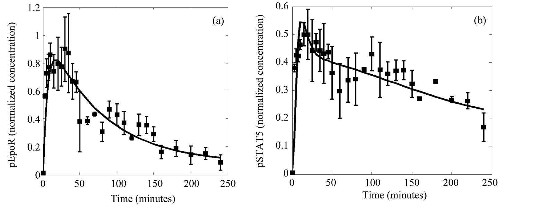
Figure 6. Data fitting of the selected solution for the observables. (a) Activated EpoR. (b) Activated cytosolic STAT5. The quantitative data with error bars obtained from experiments (points) are compared with the solution of the model identification process (lines).
Finally, it should be noted that the proposed GA can lead to an early local optimum. However, this has been prevented by providing a great diversity of the population. This is done through the insertion of three different selection processes: one to choose the individuals from which the new population will be generated by mutation and crossing; one at the moment of the local search; and a last one when choosing the elements of the following generation (Figure 1). In this way there exists a high probability to choose individuals with objective functions distant from the optimum and thus making the search space sampling more effective.
5. Conclusions
The proposed method for parameters estimation (MGA) showed better performance, both in presence and in absence of noise, compared with other parameter estimation algorithm (SGA and SA). Furthermore, leading an early local optimum can be prevented by providing great population diversity. This procedure can be changed dealt changing the selection processes.
MGA is slower than SGA and SA reaching the convergence, but this limitation is compensated by its greater efficiency in finding objective values closer to the global optimum.
Acknowledgements
The authors gratefully acknowledge Dr Julio Vera for their helpful observations. This work was funded by research Grants from Spanish MICINN, Ref. No. BIO2011-29233-C02-02 and ACIISI Project PIL2070901.
NOTES
*Corresponding author.