Using GIS Data to Build Informed Virtual Geographic Environments (IVGE) ()
1. Introduction
Modern geography techniques play an irreplaceable role in exploring temporal-spatial patterns and dynamic processes, and understanding the relationships between geographic features, objects, and actors in the real world. Studying these relationships is fundamental and comprehensive geographical analysis often requires the integration of different disciplines at various scales. By using a variety of different techniques, it is possible to produce virtual reality representations, integrated models, simulations, forecasts and evaluations of the geographic environment. Therefore, the Virtual Geographic Environment (VGE) can be a useful tool for understanding the evolutionary process, temporal-spatial patterns, driving mechanisms, and the direction of succession in the real environment. Current VGE techniques, including three-dimensional (3D) techniques, have extended the potential applications of geographic modeling. The ability of VGE to depict past, present, and future geographic environments has been of particular importance [1].
Traditional methods for extracting and expressing spatial information can be modified to better suit development in the field of geographic modeling [2]. Through using geographic analytical modeling and visualization techniques, VGE can be used to perform geographic analysis, simulate geographic phenomena, represent and predict changes in the geographic environment, and evaluate the influence of human activities on the environment [3]. By using VGE to share ideas, people can cooperate and coordinate their work on geographic objects and phenomena, resulting in more advanced methods of designing and transforming the world (Figure 1). VGE will become increasingly important in geography in the future [2].
In this paper, we propose a novel approach to modeling VGE which deals with all these constraints. Our approach provides an exact representation of the geographic environment using vector data and including elevation. This representation is organized as a topological graph, enhanced with data integrating both quantitative (geometry) and qualitative information (zones such as roads and buildings). Moreover, our approach is directed to efficient spatial reasoning like path planning for crowd simulation (Figure 2). Hence, we also address the performance issue when exploiting such environments.

Figure 1. 3D city models of East Berlin.

Figure 2. The proposed architecture to generate an IVGE.
We call our model an Informed Virtual Geographic Environment (IVGE) because it is close to standard VGE applications while addressing additional information management issues. IVGE data are directly extracted and computed from standard GIS vector files. It is a one-time automated process based on a Constrained Delaunay Triangulation (CDT) technique [4]. The produced IVGE contains spatial information which can be enhanced thanks to a geometric abstraction method. Finally, the IVGE can either be saved for future use or be exported to a GIS vector file.
The remainder of this chapter finishes with an overview on spatial reasoning and GIS data followed by a discussion of related works on GIS data and the representation of virtual environments. In Section 3, we present our approach to creating an IVGE from GIS data. Section 4 depicts a way to enhance the IVGE information by automatically associating semantics with surfaces based on their boundaries. Next, Section 5 presents two additional information enhancements based on a geometrical abstraction: first, by filtering potential elevation errors related to the input data; second, by qualifying elevation with additional semantics which are associated with specific areas in the environment. Then, Section 6 presents some results obtained by applying our approach to an urban environment. Finally, we provide a summary of this paper and present future work.
2. Spatial Reasoning and GIS Data
Spatial reasoning is a research area with applications in several domains such as crowd simulation and robotics. Reasoning about space does not only require appropriate computation algorithms, but also an efficient description of the spatial environment. Indeed, such a description must represent the geometrical information which corresponds to geographic features. Moreover, this representation must qualify space by associating semantics to geographic features in order to allow spatial reasoning. A Geographic Information System (GIS) is a system of hardware, software and procedures used to facilitate the management, manipulation, analysis, modeling, representation and display of georeferenced data to solve complex problems regarding planning and management of resources [5]. GISs have emerged in the last decade as an essential tool for urban and resource planning and management [6]. Their capacity to store, retrieve, analyze, model and map large areas with huge volumes of spatial data has led to an extraordinary proliferation of applications [5]. GISs offer two data models to describe a geographic environment: raster and vector data representations [7].
2.1. Raster Model
The raster representation of GIS data is a method for the storage, processing and display of spatial data [8]. Each area is divided into rows and columns, which form a regular grid structure [7]. Each cell must be rectangular in shape, but not necessarily square [6]. Each cell within this matrix contains location coordinates as well as an attribute value [8]. The spatial location of each cell is implicitly contained within the ordering of the matrix [9]. Areas containing the same attribute value are recognized as such, however, raster structures cannot identify the boundaries of such areas as polygons [6]. Raster data are an approximation of the real world where spatial data are expressed as a matrix of cells, with spatial position implicit in the ordering of the pixels [9]. With the raster data model, spatial data are not continuous but divided into discrete units [8]. This makes raster data particularly suitable for certain types of spatial operation, for example overlays or area calculations. Raster structures may lead to increased storage in certain situations, since they store each cell in the matrix regardless of whether it is a feature or simply empty space.
2.2. Vector Model
The vector format is defined by the vector representation of its geographic data [10]. Vector storage implies the use of vectors (directional lines) to represent a geographic feature [11]. Vector data is characterized by the use of sequential points or vertices to define a linear segment. Each vertex consists of X and Y coordinates [8]. Vector lines are often referred to as arcs and consist of a string of vertices terminated by a node [6]. A node is defined as a vertex that starts or ends an arc segment. Point features are defined by one coordinate pair, a vertex. Polygonal features are defined by a set of closed coordinate pairs [7]. In vector representation, the storage of the vertices for each feature is important, as well as the connectivity between features, e.g. the sharing of common vertices where features connect [9].
GIS offer two ways to describe an environment: grid and vector representations. Grids have several drawbacks such as the difficulty to balance accuracy and memory use, making them unusable for the precise exploitation of large scale environments. Vector layers are scalable, but it is difficult to manipulate the stored data in order to simply retrieve pieces of information or to merge data with different semantics. Moreover, while GIS data are stored in a quantitative way which suits to exact calculations, spatial reasoning often needs to manipulate qualitative information. For example, when considering a slope in a landscape, it is simpler and faster to qualify it by an attribute that takes the values light or steep rather than to directly use its angle value with respect to the horizontal plane. This process of qualification, which associates semantics with quantitative intervals of values, greatly simplifies the description and validation of reasoning mechanisms. Moreover, the slope example illustrates another requirement of spatial reasoning which is poorly addressed in the literature: providing a way to handle terrain’s elevations. Indeed, a real environment is rarely flat and ignoring this information would greatly decrease the quality of spatial reasoning.
3. Related Work
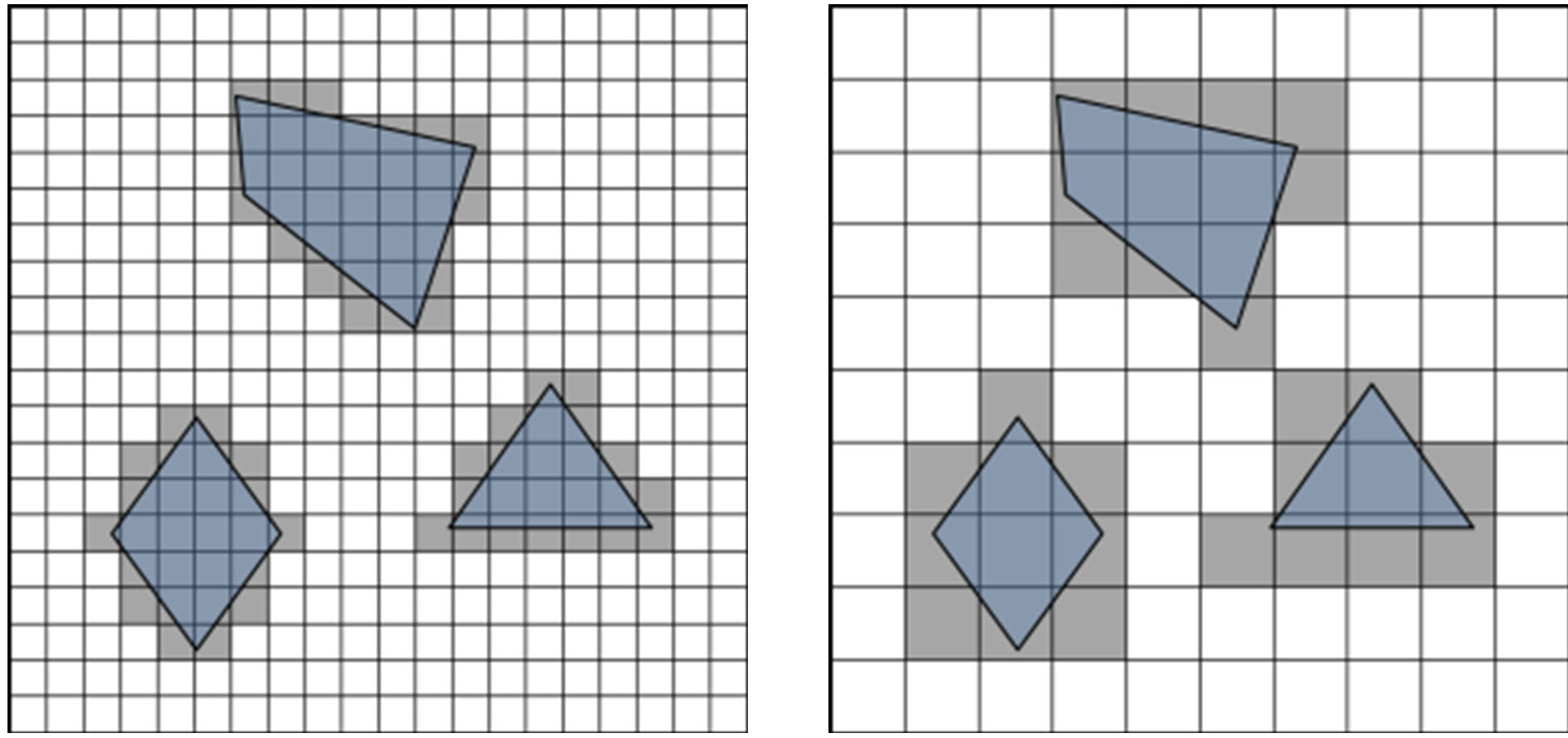
GIS data are usually available in either raster or vector formats. The raster format subdivides the space into regular square cells, called boxes, associated with space related attributes. This approach generally presents average quantitative data whose precision depends on the scale of the representation. In contrast, the vector format exactly describes geographic information without constraining geometric shapes, and generally associates one qualitative data with each shape. Such data are usually exploited by a VGE in two ways [3]: the grid method and the exact geometric subdivision. The grid method is the direct mapping of the raster format [12], but it can also be applied to the vector format (Figure 3(a)). This discrete representation can be used to merge multiple semantic data [13], the locations where to store these data being predefined by the grid cells. The main drawback of the grid method is related to a loss in location accuracy [1], making it difficult to accurately position any information which is not aligned with the subdivision. Another drawback arises when trying to precisely represent large environments using a grid: the number of cells tends to increase dramatically, which makes the environment exploitation very costly [14]. The grid-based method is mainly used for animation purposes [15] and large crowd simulations [16] because of the fast data
 (a)
(a) (b)
(b)
Figure 3. Two common cell decomposition techniques: (a) approximate decomposition by grids considering two resolutions. White boxes are free, grey are obstacles; (b) exact decomposition using CDT.
access it provides.
The second method, called exact geometric subdivision, consists in subdividing the environment in convex cells using the vector format as an input. The convex cells can be generated by several algorithms, among which the most popular is the Constrained Delaunay Triangulation (CDT) [17]. This produces triangles while keeping the original geometry segments which are named constraints (Figure 3(b)). The first advantage of the exact subdivision method is to preserve the input geometry, allowing accurately manipulating and visualizing the environment at different scales. Another advantage of this approach is that the number of produced cells only depends on the complexity of the input shapes, but not on the environment’s size and scale as it is the case with the grid method [18]. The main drawback of this approach is the difficulty to merge multiple semantic data for overlapping shapes. Moreover, this method is generally used to represent planar environments because the CDT can only handle 2D geometries [19]. This method tends to be used for crowd microscopic simulations [2] where motion accuracy is essential.
Both VGE representations, approximate and exact, can be enhanced by an abstraction process. The first goal of an abstraction is to improve the performance of the algorithms based on the environment description, such as path planning, by reducing the number of elements used to describe the environment. The usual abstraction model for grids is mainly geometric: the quadtree groups four boxes of the same kind to create a higher level cell [20]. When considering the exact decomposition, an abstraction is generally based on topological properties rather than on purely geometric ones. Indeed, the exact cell subdivision generates connected triangles which can be manipulated as the nodes of a topological graph. This graph can then be abstracted by grouping the nodes, producing a new graph with fewer nodes [21]. For example, Figure 4 shows an abstraction which is only based on the nodes’ number of connections c: isolated (c = 0), deadend (c = 1), corridor (c = 2), and crossroad (c = 3). A topological graph can be used for spatial reasoning, like path planning, thanks to traversal algorithms. These algorithms benefit of the abstraction by traversing first the more abstracted graph, and then by refining the computation in the sub-graphs until reaching the graph of the spatial subdivision [22]. This exploitation points out a new need for an abstracted graph which is less addressed in literature: it must contain the minimal information necessary to make a decision. For example, if the width of a path is relevant for a path planning algorithm, this information must be accessible in all the abstracted graphs; if not, the evaluation would be greatly distorted compared to a un-abstracted graph.
Two kinds of information can be stored in the description of an IVGE. Quantitative data are stored as numerical values which are generally used to depict geometric properties (path’s width of 2 meters) or statistical values (density of 2.5 persons per square meter). Qualitative data are introduced as identifiers which can be a reference to an external database or a word with an arbitrary semantic, called a label.
Such labels can be used to qualify an area (a road or a building) or to interpret a quantitative value (a narrow passage or a crowded place). An advantage of interpreting quantitative data is to reduce a potentially infinite set of inputs to a discrete set of values, which is particularly useful to condense information in successive abstraction levels to be used for reasoning purposes.
The approach we propose is based on an exact representation whose precision allows realistic applications like crowds’ micro-simulations. We will briefly describe how to obtain such a representation since it has already been presented in [16]. We will then show how the obtained topological graph can be improved in two ways. First, by propagating input qualitative information from the arcs of the graph to the nodes, this allows for example to deduce the internal parts of the buildings or of the roads in addition to their outline. Second, we propose a novel approach of information extrapolation using a onetime spatial reasoning process based on a geometric abstraction. This second technique can be used to fix input elevation errors, as well as to create new qualitative data relative to elevation variations. These data are stored as additional semantics bound to the graph nodes, which can subsequently be used for spatial reasoning.
4. Automated Generation of IVGE
We propose an automated approach to compute the data directly from vector format GIS data. This approach is based on three stages which are detailed in this section (Figure 5): Input data selection, spatial decomposition, and maps unification.
The first step of our approach, the inputting data selection is the only one requiring human intervention. The various vector data selected which will be used to build

Figure 4. Topologic abstraction of virtual environments.

Figure 5. A flow chart illustrating the automated generation of IVGE.
the IVGE. The only restrictions concerning these data are that they need to respect the same scale and be equally geo-referenced. The input data can be organized in two categories. First, elevation layers contain geographical marks indicating absolute terrain elevations. Since we consider the creation of 2.5D, a given coordinate cannot have two different elevations, prohibiting the representation of tunnels for example. Moreover, several elevation layers can be specified, the model being able to merge them automatically. Second, semantic layers are used to qualify various features of the geographic space. As shown in Figure 4, each layer indicates the geographic boundaries of a set of features having identical semantics, such as roads and buildings. The boundaries of the features can overlap between two layers, our model is able to merge this information.
The second step of our method, spatial decomposition, consists of obtaining an exact spatial decomposition of the input data in cells. This process uses a Delaunay triangulation and is entirely automatic. It and can be divided into two parts in relation to the previous phase. First, an elevation map is computed, corresponding to the triangulation of the elevation layers. All the elevation points of the layers are injected in a 2D triangulation, the elevation is considered as an additional datum. This process produces an environment subdivision composed of connected triangles. Such a subdivision provides information about coplanar areas: the elevation of any point inside the environment can be deduced thanks to the elevation of the three vertices of the corresponding triangle. Second, a merged semantics map is computed, which corresponds to a Constrained Delaunay Triangulation (CDT) of the semantic layers. Indeed, each segment of a semantic layer is injected as a constraint which keeps track of the original semantic data thanks to an additional datum. Consequently, the resulting map is a merging all input semantics: each constraint represents as many semantics as the number of input layers containing it.
In the third step, the two maps previously obtained are merged. This phase corresponds to the mapping of the 2D merged semantic map on the 2.5D elevation map in order to obtain the final 2.5D elevated merged semantics map. First, a preprocessing is carried out on the merged semantics map in order to preserve the elevation precision inside the unified map. Indeed, all the points of the elevation map are injected in the merged semantics triangulation, and create new triangles. Then, a second process elevates the merged semantics map. The elevation of each merged semantics point P is computed by retrieving the triangle T of the elevation map whose 2D projection contains P. Once T is obtained, the elevation is simply computed by projecting P on the plane defined by T using the Z axis. When P is outside the convex hull of the elevation map, no triangle can be found and the elevation cannot be directly deduced. In this case, we use the average height of the points of the convex hull which are visible from P.
5. Semantic Information Management
The obtained results of the importation technique emphasize qualified areas by defining the semantics of their boundaries. But these informed boundaries are difficult to exploit when dealing with the semantics associated with a position. For example, it is difficult to check if a position is inside a building. This is why we propose to enhance the information provided by spreading the boundaries’ semantics to the cells. Three related processes are necessary, and explained in the following subsections: graph analysis, potential conflicts resolution, and semantics assignment.
5.1. Graph Analysis
The graph analysis is a traversal algorithm which explores the environmental graph while qualifying the cells towards a given semantic. This algorithm is applied to the entire graph one time for each semantic to propagate. While exploring the graph, the algorithm collects three kinds of cells which are stored in three container structures for future use: Inside, Outside and Conflict. Cells are within an area delimited by borders associated to the propagated semantic. Outside cells are outside any area defining the propagated semantic. Conflict (C) cells are both qualified inside and outside by the algorithm. NonConflict (NC) cells are either qualified inside or outside by the algorithm. Three parameters influence the traversal: 1) the semantic sem to propagate. 2) a set of starting cells, indicating where to start the exploration of the graph; a set is provided instead of a single cell in order to be able to manage disconnected graphs. 3) a boolean value startin indicating whether the semantic must be assigned to the starting cells or not. The recursive algorithm is detailed in Figure 6.
5.2. Resolution of Conflicts
After each graph traversal, we must deal with the cells that are potentially in conflict. Indeed, these cells must be assigned to either the Inside or the Outside container in order for the system to continue with the next phase. Cells are in conflict when the shapes of two input features with the same semantic share a segment. Two alternative methods are proposed: 1) a fast assignment where the conflicting cells are arbitrarily transferred to one of the target containers, and 2) a deductive assignment where an algorithm selects the best option based on geometric considerations. The arbitrary assignment is used when the internal details of a shape are not relevant for the target application. The deductive assignment is used when the internal details of a shape are relevant. Both methods are carried out in two steps: 1) a local conflicting graph extraction which is the same for both methods, and 2) a decision step which is specific to each method. The local conflicting graph extraction collects all the cells surrounding a conflicting cell, but only if they are reachable through a border which is not marked by the propagated semantic. Each orange zone in Figure 6 shows an extracted local conflicting graph. Every time a cell is discovered, it is transferred from the global container Conflict to a local container. Then, the algorithm recursively explores the neighbors which are reachable through a border which is not marked by the propagated semantic, transferring them to the local container. At the end, the algorithm obtains a set of local conflict containers, corresponding to the amount of local graphs considered in conflict.
The decision part of the arbitrary assignment only consists in transferring the local conflicting cells to one of the Inside or the Outside containers. The decision part of the deducing algorithm is based on geometric considerations. If the local conflicting zone is mainly surrounded by Outside cells, then the conflict is resolved as Inside, and vice versa. The conflict management algorithm is described in Figure 7.
5.3. Semantics Assignment
The last step of the semantic propagation consists in assigning the final semantics to the cells. The process is very simple: each propagated semantic is assigned to all the corresponding Inside cells. One can notice that some cells may have multiple semantics when they are present in more than one Inside container. Additionally, it is possible to keep track of the Outside cells by assigning them

Figure 7. Semantic propagation and conflict management algorithm.
a negative semantic, as for example in order to know what is road in the environment and what is not.
Finally, an optional process can be performed to remove the borders’ semantics of some detected conflicting cells. Indeed, such borders may distort some spatial reasoning algorithms. For example, when considering road borders as obstacles to plan a path, a simulated vehicle would not be able to go through some passageways. After resolution, the semantic of the problematic borders is removed, making them crossable. These problematic borders are the ones which are marked with a propagated semantic and which connect two Inside cells. One can note that only the cells previously detected as conflicting need to be tested.
Spatial decomposition subdivides the environment into convex cells. Such cells encapsulate various quantitative geometric data which are suitable for accurate computations. Since geographic environments are seldom flat, it is important to consider the terrain’s elevation, which is quantitative geometric data. Moreover, while elevation data are stored in a quantitative way which suits exact calculations, spatial reasoning often needs to manipulate qualitative information. Indeed, when considering a slope, it is obviously simpler and faster to qualify it using an attribute such as light and steep rather than using numerical values. However, when dealing with large scale geographic environments, handling the terrain’s elevation, including its light variations, may be a complex task. To this end, we propose an abstraction process that uses geometric data to extract the average terrain’s elevation information from spatial areas. The objectives of this Geometric Abstraction are threefold [23]. First, it aims to reduce the amount of data used to describe the environment. Second, it helps detect anomalies, deviations, and aberrations in elevation data. Third, the geometric abstraction enhances the environmental description by integrating qualitative information characterizing the terrain’s elevations. In this section, we first present the algorithm which computes the geometric abstraction. Then, we describe two processes which use the geometric abstraction: Filtering elevation anomalies and Extracting elevation semantics.
6.1. Geometric Abstraction Algorithm
The geometric abstraction process gathers cells in groups according to a geometric criterion: we chose the coplanarity of connex cells in order to obtain uniform elevation areas. The algorithm takes advantage of the structure obtained thanks to the IVGE generation process.
The aim of this algorithm is to group cells which verify a geometric criterion in order to build groups of cells. A cell corresponds to a node in the topological graph. A node represents a triangle generated by the CDT spatial decomposition technique. A cell is characterized by its boundaries, neighboring cells, and surface as well as its normal vector which is a vector perpendicular to its plan Figure 8(a).
A group is a container of adjacent cells. The grouping strategy of this algorithm is based on a coplanarity criterion which is assessed by computing the difference between the normal vectors of two neighboring cells or groups of cells (Figure 8(a)). Since a group is basically composed of adjacent cells it is obvious to characterize a group by its boundaries, its neighboring groups, its surface, as well as its normal vector. However, the normal vector of a group must rely on an interpretation of the normal vectors of its composing cells. In order to compute the normal vector of a group, we adopt the areaweight normal vector [24] which takes into account the unit normal vectors of its composing cells as well as their respective surfaces. The area-weight normal vector of a group  is computed using:
 (1)
(1)
where Sc denotes the surface of a cell c and Nc its unit normal vector. Hence, thanks to the area-weight normal vector we are able to compute a normal vector for a group based on the characteristics of its composing cells. The geometric abstraction algorithm uses two input parameters: 1) a set of starting cells which act as access points to the graph structure, and 2) a gradient parameter which corresponds to the maximal allowed difference between cells’ inclinations. Indeed, two adjacent cells are considered coplanar and grouped together when the angle between their normal vectors (α in Figure 8(b)) is lesser than gradient.
The analysis of the resulting groups helps to identify anomalies in elevation data. Such anomalies need to be fixed in order to build a realistic virtual geographic environment. Furthermore, the average terrain’s elevation which characterizes each group is quantitative data described using area-weighted normal vectors. Such quantitative data are too precise to be used by qualitative spatial reasoning. For example, when considering a slope in a landscape, it is simpler and faster to qualify it using a simple attribute that takes the values light and steep rather than to express it using the angle value with respect to the horizontal plane. Hence, a qualification process which aims to associate semantics with quantitative intervals of values characterizing a group’s terrain inclinations would greatly simplify spatial reasoning mechanisms. In addition, in order to fix anomalies in elevation data and to qualify the groups’ terrain inclinations we propose to apply a technique to improve the geometric
 (a)
(a) (b)
(b)
Figure 8. (a) Illustration of two coplanar cells; (b) Unit normal vectors.
abstraction of the VGE. The geometric abstraction allows improving IVGE by filtering the elevation anomalies, qualifying the terrain’s elevation using semantics and integrating such semantics in the description of the geographic environment.
A detailed description of the geometric abstraction algorithm as well as GIS data filtering and elevation qualification processes are provided in [23]. The geometric abstraction is built using a graph traversal algorithm. It groups cells based on their area-weighted normal vectors (Figure 8(b)). The objectives of the geometric abstraction are threefold. First, it qualifies the terrain’s elevation of geographic environments to simplify spatial reasoning mechanisms. Second, it helps identifying and fixing elevation anomalies in initial GIS data. Third, it enriches the description of geographic environments by integrating elevation semantics.
6.2. Filtering Elevation Anomalies
The analysis of the geometric abstraction may reveal some isolated groups which are totally surrounded by a single coherent group. These groups are characterized by a large difference between their respective area-weighted normal vectors. Such isolated groups are often characterized by their small surfaces and can be considered anomalies, deviations, or aberrations in the initial elevation data. The geometric abstraction process helps to identify and allows automatically filtering such anomalies thanks to a two phase process.
First, isolated groups are identified (Figure 9(a)). The identification of isolated groups is based on two key parameters: 1) the ratio between the surface of surrounded and surrounding groups, and 2) the difference between
 (a)
(a) (b)
(b)
Figure 9. Profile section of anomalous isolated groups (red color) adjusted to the average elevation of the surrounding ones (yellow color).
the area-weighted normal vectors of the surrounded and surrounding groups. Second, these isolated groups are elevated at the average level of elevation of the surrounding ones (Figure 9(b)). In fact, the lowest and the highest elevations of the isolated group are computed. Then, the elevations of all the vertices of isolated grp are updated using the average between the lowest and highest elevation. As a consequence, we obtain more coherent groups in which anomalies of elevation data are corrected.
6.3. Extracting Elevation Semantics
The geometric abstraction algorithm computes quantitative geometric data describing the terrain’s inclination. Such data are stored as numerical values which allow to accurately characterize the terrains’ elevations.
However, handling and exploiting quantitative data is a complex task as the volume of values may be too large and as a consequence difficult to transcribe and analyze. Therefore, we propose to interpret the quantitative data of the terrain’s inclination by qualifying the areas’ elevations. Semantic labels, called semantics elevation, are associated to quantitative intervals of values that represent the terrain’s elevation. In order to obtain elevation semantics we propose a two steps process taking advantage of the geometric abstraction: 1) a discretization of the angle between the weighted normal vector Ng of a group g and the horizontal plane, 2) an assignment of semantic information to each discrete value which qualifies it. The discretization process can be done in two ways: a customized and automated approach.
The customized approach qualifies the terrain’s elevation and requires that the user provides a complete specification of the discretization. Indeed, the user needs to specify a list of angle intervals as well as their associated semantic attributes. The algorithm iterates over the groups obtained by the geometric abstraction. For each group grp, it retrieves the terrain inclination value I. Then, this process checks the interval bounds and determines in which one falls the inclination value I. Finally, the customized discretization extracts the semantic elevation from the selected elevation interval and assigns it to the group grp. For example, let us consider the following inclination interval and the associated semantic elevations: f([10; 20]; gentle slope); f([20; 25]; steep slope). Such a customized specification associates the semantic elevation “gentle slope” to inclination values included in the interval [10; 20] and the semantic elevation “steep slope” to inclination values included in the interval [20; 25]. The automated approach only relies on a list of semantic elevations representing the elevation qualifications. Let N be the number of elements of this list, and T be the total number of groups obtained by the geometric abstraction algorithm. First, the automated discretization orders groups based on their terrain inclination. Then, it iterates over these ordered groups and uniformly associates a new semantic elevation from the semantics set of each T = N processed groups. For example, let us consider the following semantic elevations: gentle; medium and steep. Besides, let us consider an ordered set of groups S which may be composed of six groups of cells.
Let us compare these two discretization approaches. On the one hand, the customized discretization process allows one to freely specify the qualification of the terrain’s elevations. However, qualifications resulting from such a flexible approach deeply rely on the correctness of the interval bounds’ values. Therefore, the customized discretization method requires having a good knowledge of the terrain characteristics in order to guarantee a valid specification of inclination intervals. On the other hand, the automated discretization process is also able to qualify groups’ elevations without the need to specify elevation intervals’ bounds. Such a qualification usually produces a visually uniformed semantic assignment. This method also guarantees that all the specified semantic attributes will be assigned to the groups without a prior knowledge of the environment characteristics.
6.4. Enhancing the Geometric Abstraction
The geometric abstraction algorithm produces groups that are built on the basis of their terrain’s inclination characteristics. Thanks to the extraction of elevation semantics, the terrain’s inclination is qualified using semantic attributes and associated with groups and with their cells. Because of the game of the classification intervals, adjacent groups with different area-weighted normal vectors may obtain the same elevation semantic. In order to improve the results provided by the geometric abstraction, we propose a process that merges adjacent groups which share the same semantic elevation. This process starts by iterating over groups. Then, every time it finds a set of groups sharing an identical semantic elevation, it creates a new group. Next, cells composing the adjacent groups are registered as members of the new group. Finally, the area-weighted normal vector is computed for the new group. Hence, this process guarantees that every group is only surrounded by groups which have different semantic elevations (Figure 10). In this section, we proposed a geometric abstraction process as well as three heuristics which take advantage of this process. The geometric abstraction is built using a graph traversal algorithm. It groups cells based on their areaweighted normal vectors. The objectives of the geometric abstraction are threefold. First, it qualifies the terrain’s elevation of geographic environments to simplify spatial reasoning mechanisms. Second, it helps identify and fix elevation anomalies in initial GIS data. Third, it enriches the description of geographic environments by integrating elevation semantics.
7. Results
The proposed environment extraction method is used to create an accurate IVGE and provides the advantages of standard GIS visualization techniques including the semantic merging of grids along with the accuracy of vector data layers. Thanks to the automatic extraction method that we propose, our system handles the IVGE construction directly from a specified set of vector format GIS files. The performance of the extraction process is very good and able to process an area such as the center part of Quebec-City, with one elevation map and five semantic layers, in less than five seconds on a standard computer (Intel Core 2 Duo processor 2.13 Ghz, 1 G RAM). The obtained unified map approximately contains 122,000 triangles covering an area of 30 km2. Besides, the necessary time to obtain the triangle corresponding to a given coordinate is negligible (less than 10−4 seconds). Moreover, the geometric abstraction produces approximately 73,000 groups in 2.8 seconds. Finally, the custom and automated discretization processes are performed respectively in 1.8 and 1.2 seconds using eight semantic elevation labels. The IVGE application provides two visualization modes for the computed data. First, a 3D view (Figure 10) allows to freely navigating the virtual environment. We propose an optional mode for this view where the camera is constrained at a given height above the ground, allowing the elevation variations to be followed when navigating. Second, we propose an upper view with orthogonal projection to represent the GIS data as a standard map. In this view the user can scroll and zoom the map (Figure 10), and can accurately view any portion of the environment at any scale. Additionally, one can select a position in the environment in order to retrieve the corresponding data (2 in Figure 10), such as the underlying triangle geometry, the corresponding height, and the associated semantics, including semantic elevation.
 (a)
(a) (b)
(b)
Figure 10. (a) 2D map visualization of the IVGE: (1) Unified map, (2) Accurate information about the selected position; (b) Results of the geometric abstraction process.
Our approach goes beyond classical grid-based visualization by combining the semantic information and the vector-based representation’s accuracy. Indeed, our topological method combines the advantages of grids and vector layers, and avoids their respective drawbacks. Moreover, this data extraction method is fully automated, being able to directly process GIS vector data. In addition, the propagation of the borders’ semantics enhances the information provided by the IVGE. As a result, both boundaries and areas are semantically qualified (roads and buildings). Besides, the geometric abstraction algorithm enriches the IVGE description by qualifying the terrain inclination characteristics of cells using semantic elevation. Finally, we have shown the suitability of this method for GIS visualization thanks to an IVGE application which allows two visualization modes: 3D for immersion purpose, and 2D to facilitate geographic data analysis.
8. Conclusion
All of the above-mentioned characteristics allow us to anticipate several applications of this work, mainly thanks to the exploitation of the topological graph. Firstwe are currently working on the application of the IVGE for crowd simulation. Indeed, this informed environment is particularly well adapted to such a domain, since it allows efficient path planning and navigation algorithms and provides useful spatial data which are needed for agents’ behaviors. However, we plan to further improve the environment description by using topological graph abstractions. This will allow us to reduce the complexity of the graph exploration algorithms, and to deduce additional properties such as the reachable areas for a human being with respect to variations of land slopes. Second, we want to append new information to the environment description in order to represent moving and stationary situated elements. These elements could be humans, vehicles, or even street signs, depending on the objectives of the virtual reality application. Our topological graph which describes the geographic environment can be extended by integrating conceptual nodes representing such elements. Thanks to the geometrical accuracy of our approach, it will be relatively easy to add this information at any position.
9. Acknowledgements
This research was supported in part by the Research Stimulus Dollars Award provided by the University of Minnesota Crookston. The author would like to thank the reviewers for their valuable comments.