A New Large Scale Instability in Rotating Stratified Fluids Driven by Small Scale Forces ()
1. Introduction
Large scale instabilities are very important in fluid dynamics. They generate vortices which play a fundamental role in turbulence and in transport processes. The characteristic dimensions of the large scale structures are greater than the typical scale of the turbulence. The turbulence is often simulated using a small scale external force. In this case, the large scale vortices are much greater than the scale of the external force. Large scale vortices are well observed in planetary atmospheres [1, 2], in numerical simulations, and in laboratory experiments [3-10]. The generation process of large scale instabilities has been studied in several papers [11-19]. In these papers, the turbulence which generates these coherent large scale structures cannot be homogenous, isotropic, or mirror invariant. A series of papers have shown that the essential mechanism which leads to the generation of large scale vortices is the lack of reflection invariance. This mechanism was called the hydrodynamic α-effect by analogy with the similar mechanism of generation of large scale magnetic fields.
Turbulence lacking reflection invariance is helical and a pseudo-scalar  appears. Nevertheless, the helicity of turbulence by itself can not generate large scale vortices. Other factors which lack reflection invariance are necessary, such as, for instance, compressibility [16,19] or temperature gradients [17,18]. Large scale instability can also appear if the turbulence lacks parity invariance (AKA effect) [12]. The helicity of the turbulence can be defined in a phenomenological way, but helicity can also be generated by an internal mechanism like rotation or buoyancy [13,15,20].
Large scale instabilities in a stratified rotating flow were studied in [21,22]. In [21], it was shown that a rotating incompressible flow with a constant temperature gradient can not display a large scale instability. In [22] the author presented large scale instabilities with a quadratic temperature gradient. In both papers, the authors used the functional averaging method. This method has some inconveniences. Especially it is impossible to make a strict hierarchy of orders as in perturbation theory. This means that it is impossible to identify the orders in which the instability appears and the ones in which it is absent. That is why the fact that the instability is absent when using the functional averaging method can not exclude its occurrence when using the rigorous asymptotic method of multi-scale development.
The occurrence of large scale instability in helical stratified turbulence was confirmed by the multi-scale development method in [23]. In that paper it was shown that the instability appears at the third order in the asymptotical development built on the small value of the Reynolds number. But in the first papers on this subject, using the functional averaging method, it was not clear in which order the instability would appear.
Direct numerical simulation of the Boussinesq Equation confirmed the existence of large scale vortex generation in stratified and rotating flows [24,25]. Sometimes the appearance of large scale vortex structures is accompanied by an inverse cascade of energy both in the threedimensional case (AKA-effect [26]), and in the quasi two-dimensional case [4,7,9,10]. One may say that the inverse cascade itself is also one of the mechanisms of the generation of large scale structures [5,27]. One of the important large scale instabilities in an incompressible fluid is the AKA effect (Anisotropic Kinetic Alpha effect) which was found in the work of Frisch, She and Sulem [11]. In this paper, the large scale instability appears under the impact of a small scale force in which parity is broken (with zero helicity). In a later paper [12], the inverse cascade of energy and the nonlinear mode of instability saturation were studied. Despite the fact that the broken parity is a more general notion than helicity, in fact, the helicity  is the widespread mechanism of symmetry breaking in hydrodynamical flows. The injection of a helical external force into a hydrodynamic system has been studied in several papers [16,19]. As a result, it was understood that a small scale turbulence that is able to generate large scale perturbations can not be simply homogeneous, isotropic, and helical [28], but must have additional special properties. In some cases, the existence of a large scale instability has been shown (a vortex dynamo or the hydrodynamic
  -effect). In the magneto hydrodynamics of a conductive fluid, the
  -effect is well known [29]. In particular, in [17] it was shown that a large scale instability exists in convective systems with small scale helical turbulence. These papers as well as the results of numerical modelling are described in detail in the review article [30], which is focused essentially on possible applications of these results to the issue of tropical cyclone origination. In this paper, we develop an analytical theory of the new large scale instability which generates large scale vortices in a stratified rotating flow with a constant temperature gradient under the action of a small scale external force which does not have any particular properties (especially it is nonhelical and it does not lack parity invariance). The force only maintains turbulent fluctuations. In other words, this force cannot display any instability. But the situation changes when both the Coriolis force and the buoyancy are added to this force. The joint action of these forces generates an internal helicity, which in turn generates an instability. The theory of this instability is developed rigourously using the method of asymptotic multi-scale development similar to what was done by Frisch, She and Sulem for the theory of the AKA effect [11]. This method allows finding the equations for large scale perturbations as the secular equations of perturbation theory, to calculate the Reynolds stress tensor and to find the instability. Our paper is organised as follows: In Section 2, we formulate the problem and the equations for the Coriolis force and the stratification in the Boussinesq approximation; In Section 3, we examine the principal scheme of the multi-scale development and we give the secular equations. In Section 4, we describe the calculations of the Reynolds stress. In Section 5, we discuss the instability and the conditions for its realization. The results obtained are discussed in the conclusions given in Section 6. The Reynolds stress and internal helicity are calculted in Appendices A and B, respectively.
2. The Main Equations and Formulation of the Problem
Let us consider the equations for the motion of an incompressible fluid with a constant temperature gradient in the Boussinesq approximation:
 (1)
(1)
 (2)
(2)
 (3)
(3)
Here,  ,
,  is the thermal expansion coefficient,
  is the constant equilibrium gradient of the temperature,
  , and
, and . The external force
  has zero divergence. Let
  be, respectively, the characteristic scale, time, amplitude of the external force, and velocity of our system. We choose the dimensionless variables

Then,
where  where R and
are respectively the Reynolds number and the Taylor number on scale .
.  represents the Prandtl number. We introduce the dimensionless temperature
 , and obtain the system of equations


Here,  is the Rayleigh number on the scale
 . Furthermore, for the purpose of simplification, we will consider the case
 . We pass to the new temperature
 , and obtain
 (4)
(4)
 (5)
(5)

We will consider as a small parameter of an asymptotic development the Reynolds number 
on the scale . Concerning the parameters
  and
and , we do not choose any range of values for the moment. Let us examine the following formulation of the problem. We consider the external force as being small and of high frequency. This force leads to small scale fluctuations in velocity and temperature against a background of equilibrium. After averaging, these quickly oscillating fluctuations vanish. Nevertheless, due to small nonlinear interactions in some orders of perturbation theory, nonzero terms can occur after averaging. This means that they are not oscillatory, that is to say, they are large scale. From a formal point of view, these terms are secular, i.e., they create the conditions for the solvability of a large scale asymptotic development. So the purpose of this paper is to find and study the solvability equations, i.e., the equations for large scale perturbations. Let us denote the small scale variables by
 , and the large scale ones by
 . The small scale partial derivative operation
 , and the large scale ones
  are written, respectively, as
and . To construct a multi-scale asymptotic development we follow the method which is proposed in [11].
3. The Multi-Scale Asymptotic Development
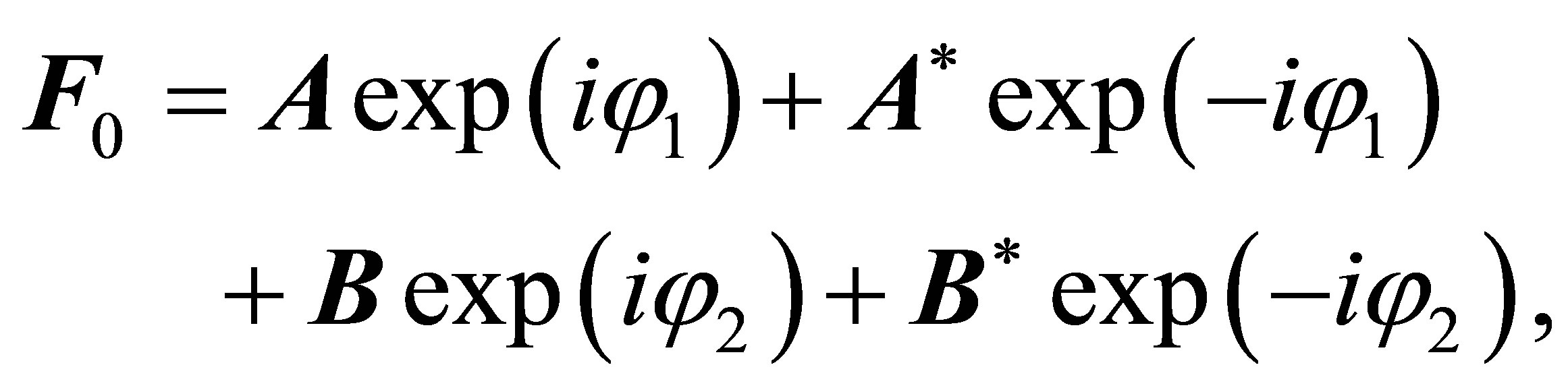
Let us search for the solution to Equations (4) and (5) in the following form:
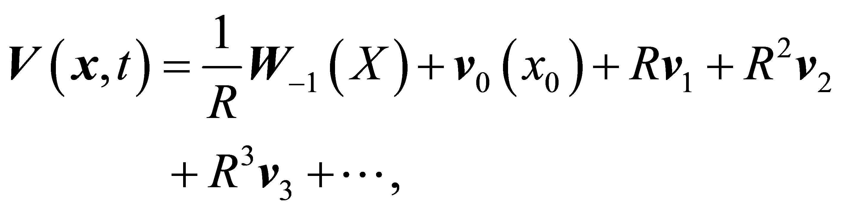 (6)
(6)
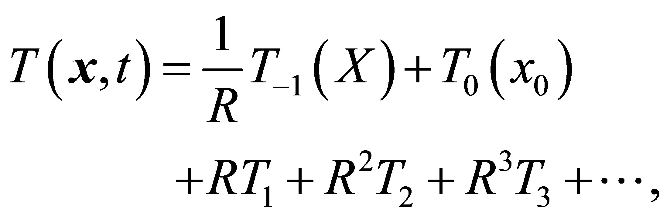 (7)
(7)
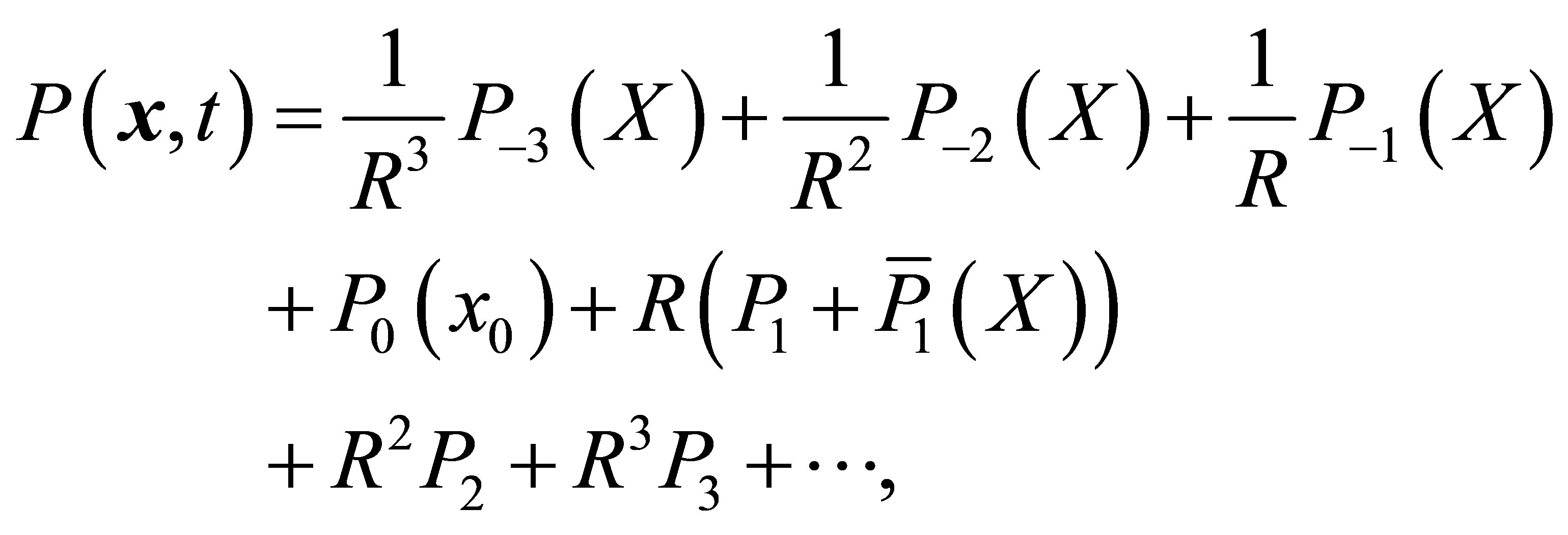 (8)
(8)
Let us introduce the following equalities:  and
and  which lead to the expression for the space and time derivatives:
 (9)
(9)
 (10)
(10)
 (11)
(11)
Using indicial notation, the system of the equation can be written as
 (12)
(12)
 (13)
(13)
 (14)
(14)
Substituting these expressions into the initial equations (4) and (5) and then gathering together the terms of the same order, we obtain the equations of the multiscale asymptotic development and write down the obtained equations up to order  inclusive. In the order
  there is only the Equation
 (15)
(15)
In order  we have the equation
 (16)
(16)
In order  we get a system of equations:
 (17)
(17)
 (18)
(18)

The system of Equations (17) and (18) gives the secular terms
 (19)
(19)
which corresponds to a geostrophic equilibrum Equation, and
 (20)
(20)
In zero order , we have the following system of equations:
 (21)
(21)
 (22)
(22)
These equations give one secular Equation:
 (23)
(23)
Let us consider the equations of the first approximation R:
 (24)
(24)
 (25)
(25)
 (26)
(26)
From this system of equations there follows the secular equations:
 (27)
(27)
 (28)
(28)
 (29)
(29)
The secular equations (27) and (29) are satisfied by choosing the following geometry for the velocity field:
 (30)
(30)
In the second order , we obtain the equations
 (31)
(31)
 (32)
(32)
 (33)
(33)
It is easy to see that there are no secular terms in this order..
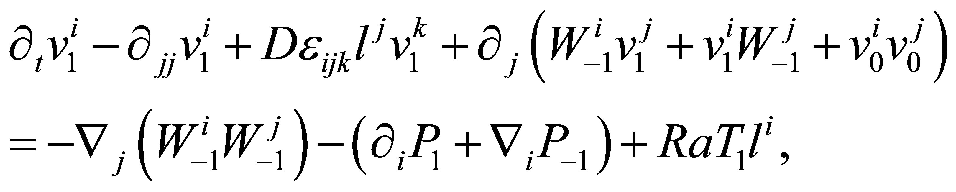
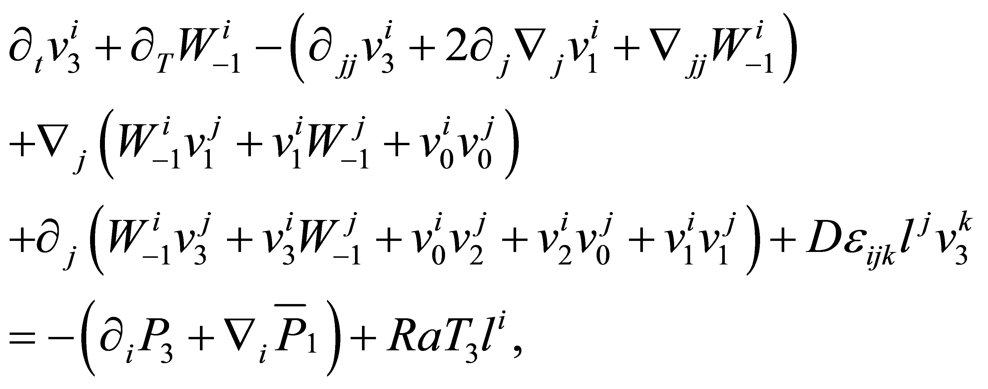
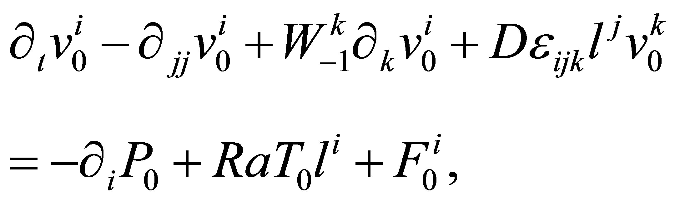
Let us come now to the most important order . In this order we obtain the equations
 (34)
(34)
 (35)
(35)
From this we get the main secular Equation:
 (36)
(36)
 (37)
(37)
There is also an Equation to find the pressure :
:
 (38)
(38)
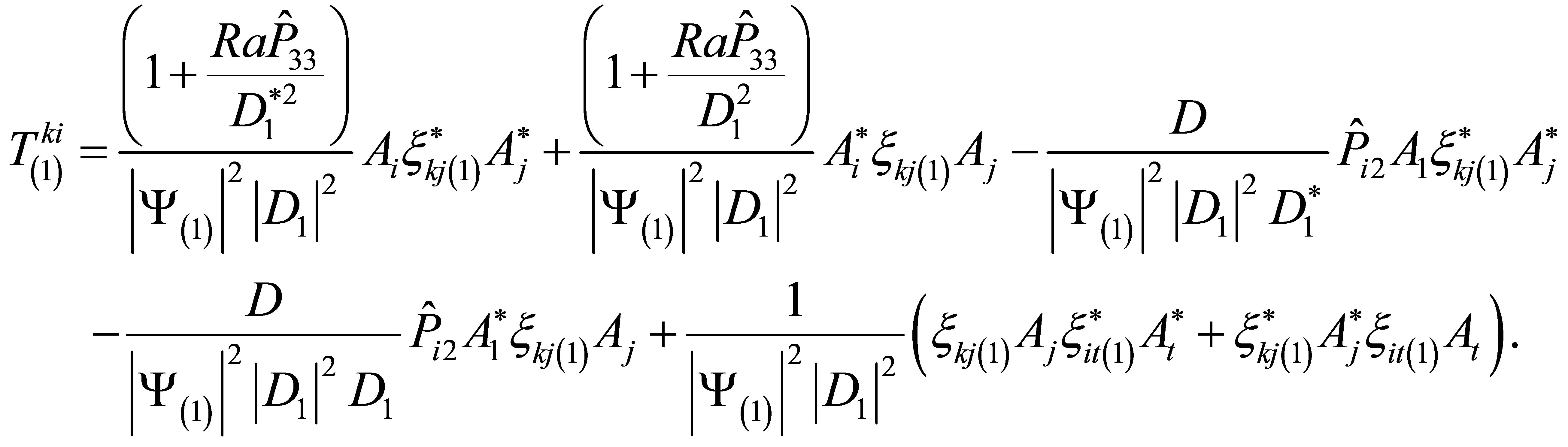
4. Calculations of the Reynolds Stresses
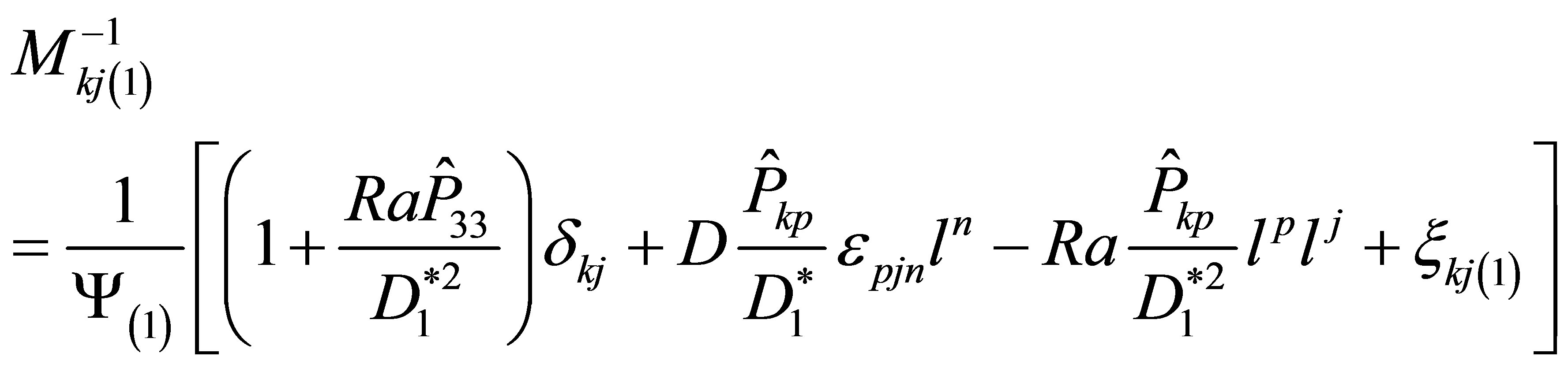
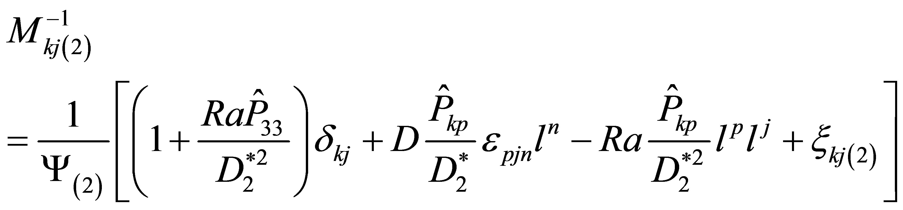
It is clear that the essential Equation for finding the nonlinear alpha-effect is Equation (36). In order to obtain these equations in closed form, we need to calculate the Reynolds stresses . First of all we have to calculate the fields of zero approximation
 . From the asymptotic development in zero order we have
 (39)
(39)
 (40)
(40)
Let us introduce the operator :
:
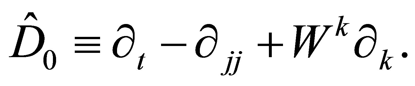 (41)
(41)
Using , we rewrite Equations (39) and (40):
 (42)
(42)
 (43)
(43)
Eliminating the temperature and pressure from Equation (42), we obtain
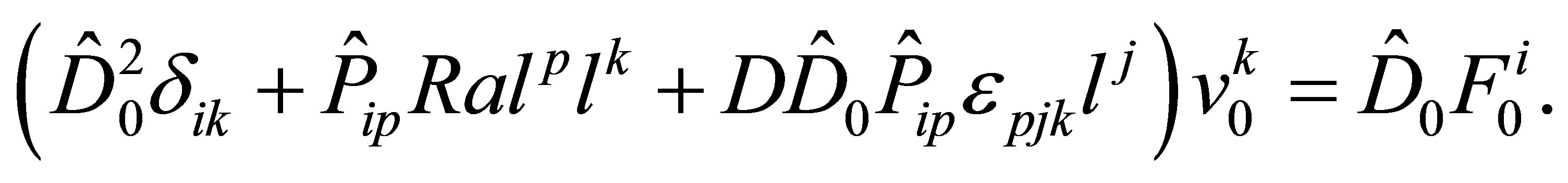 (44)
(44)
Here,  is the projection operator
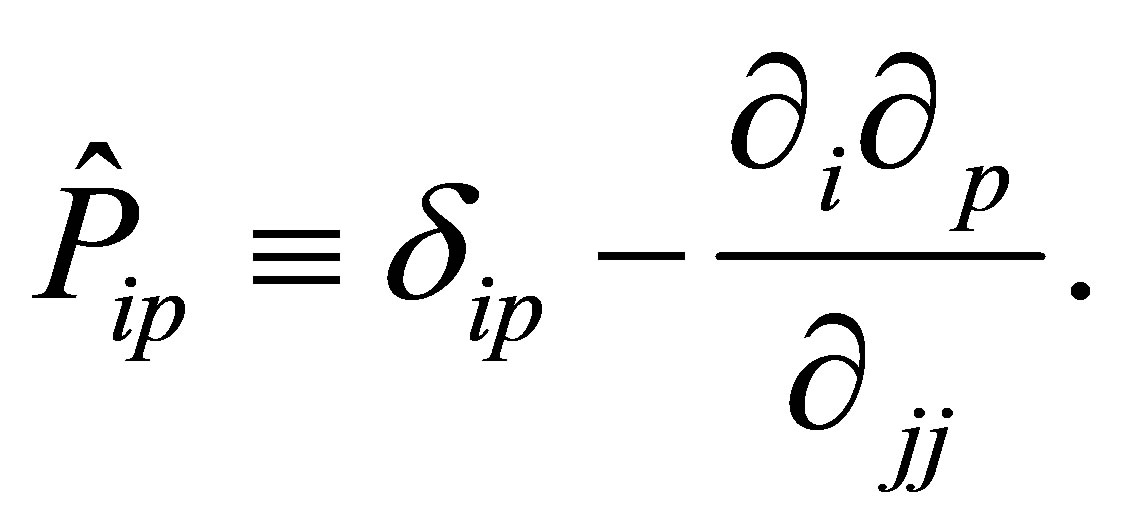
Dividing this equation by , we can write it in the form
 (45)
(45)
where  is the operator given by
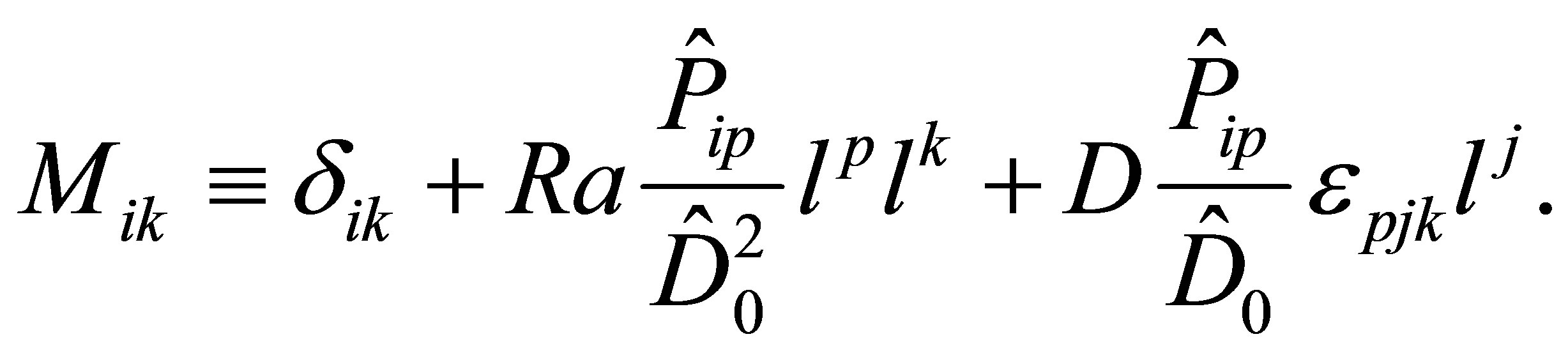 (46)
(46)
We must now determine the inverse operator 
 :
: 
After some calculation, we find
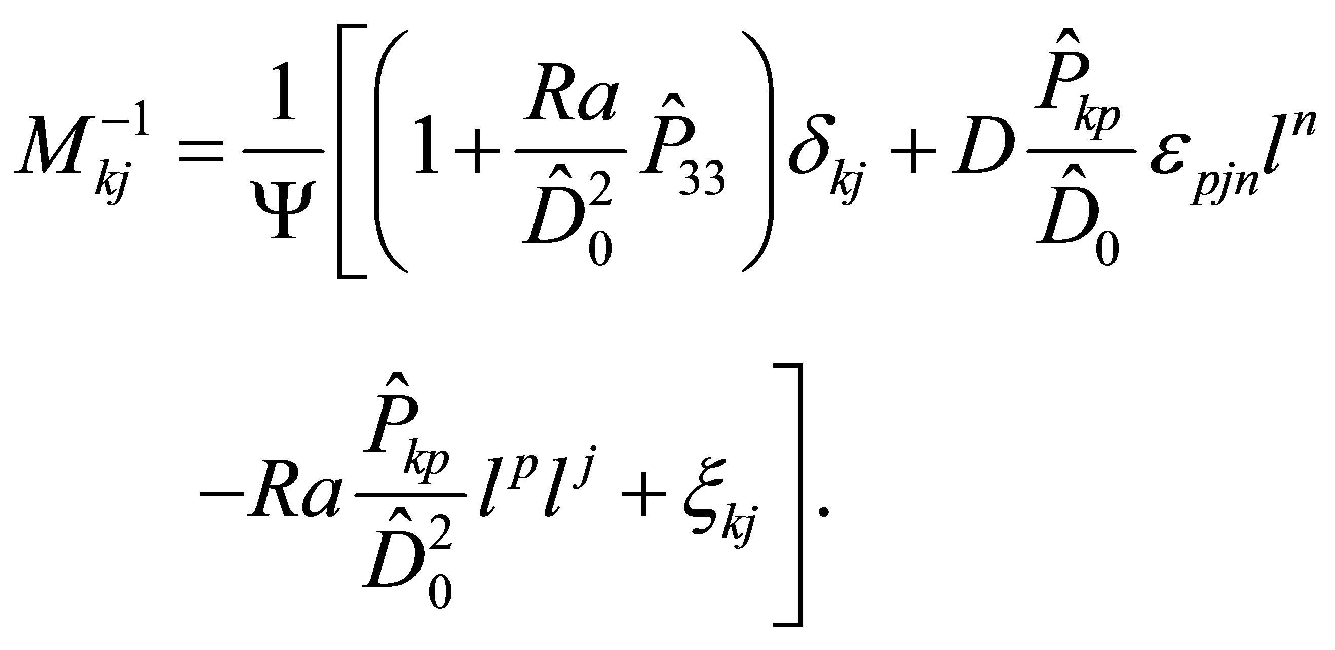 (47)
(47)
Here,
 (48)
(48)
and
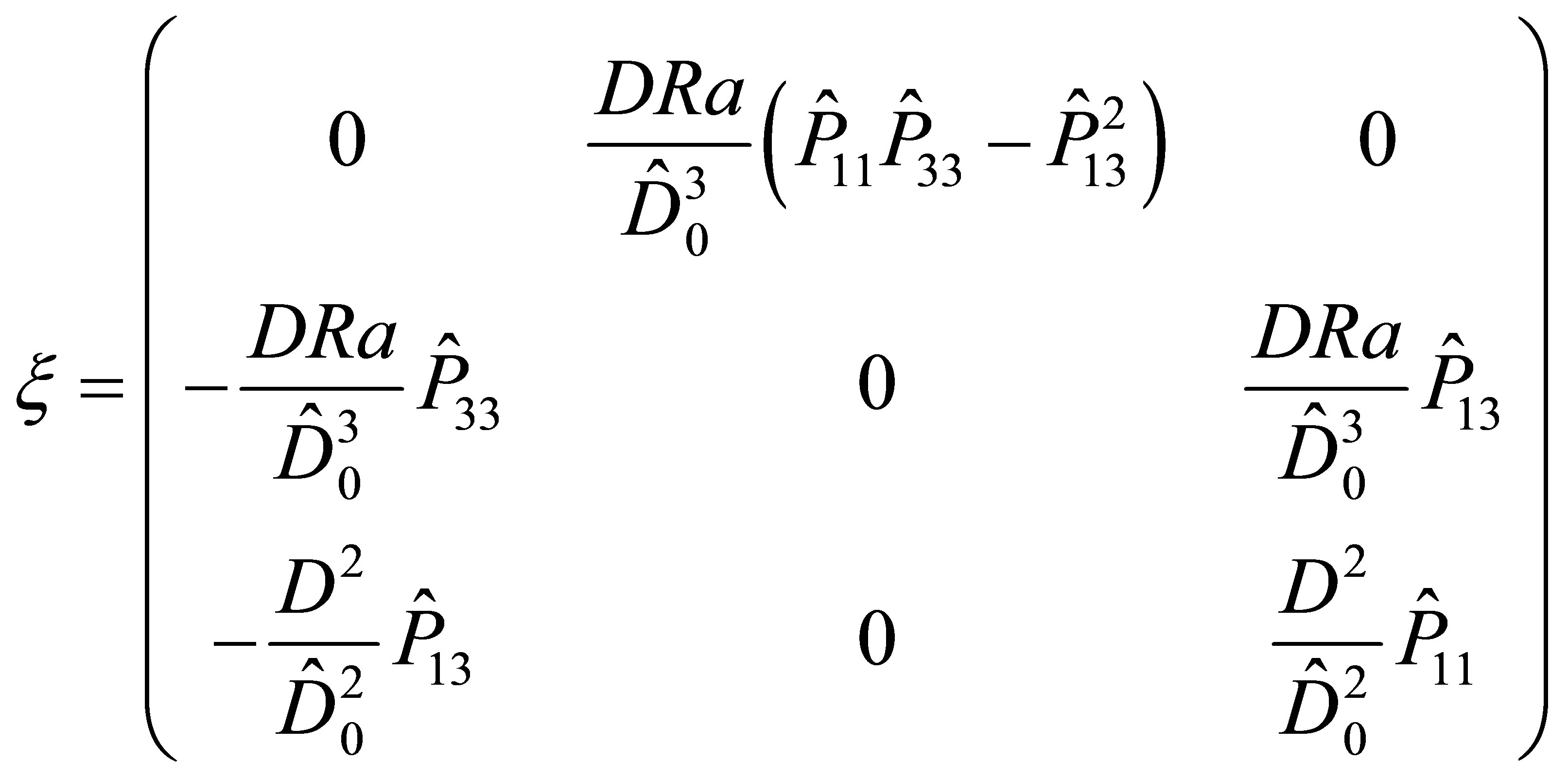
Consequently, the expression for the velocity  takes the form
 (49)
(49)
In order to use these formulas, we have to specify in explicit form the external force . Let us specify it by
 (50)
(50)
where
 (51)
(51)
or
 (52)
(52)
One can check that  and
and 
Formulas (50) and (52) allow us to easily make intermediate calculations, but in the final formulas we obviously shall take  and
and  as equal to unity, since the external force is dimensionless and depends only on the dimensionless arguments of space and time. The force (50) is physically simple and can be realized in laboratory experiments and in numerical simulations.
The force (50) can be written in complex form:
 (53)
(53)
where  and
and  have the forms
 (54)
(54)
The effect of the operator  on the proper function
  has obviously the form
 where
where  is
is
 (55)
(55)
From this it follows that
 (56)
(56)
 (57)
(57)
 (58)
(58)
 (59)
(59)
From Formulas (49) and (53), it follows that the field  is composed of four terms:
 (60)
(60)
where

Finally, we introduce the notation
 (61)
(61)
 (62)
(62)
 (63)
(63)
where . Taking into account these formulas, we can write down the velocities
  in the form
 (64)
(64)
 (65)
(65)
where
and
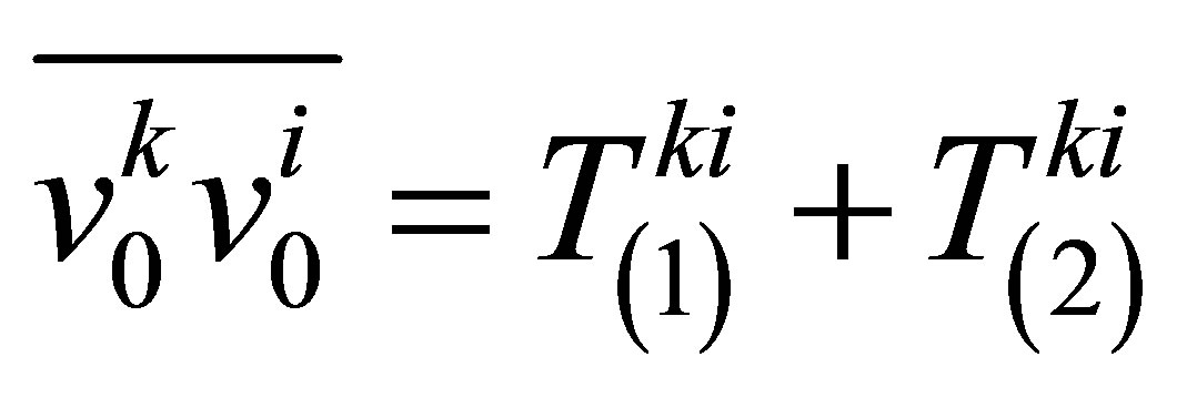
We can now calculate the Reynolds stresses:
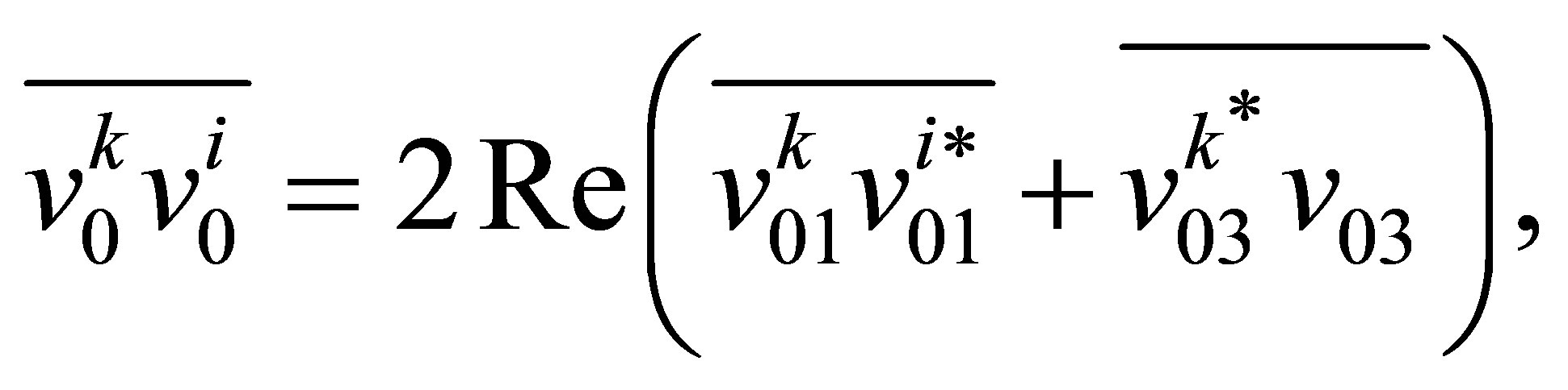 (66)
(66)
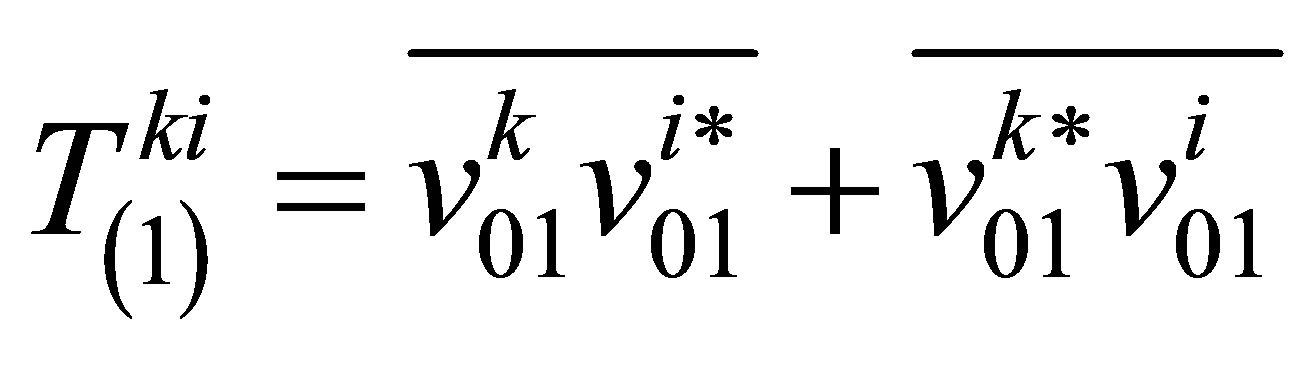
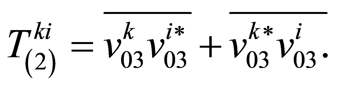
which can be decomposed into two components:
 (67)
(67)
where  and
and  can be expressed as follows:
 (68)
(68)
 (69)
(69)
Taking into account Formulas (64) and (65), we obtain

We can write down the components  and
and , which are the ones of interest:
 (70)
(70)
 (71)
(71)
 (72)
(72)
 (73)
(73)
Finally, using the following relations (we have similar formulas for  after replacing
  with
with ):
):
 (74)
(74)
 (75)
(75)
 (76)
(76)
 (77)
(77)
 (78)
(78)
 (79)
(79)
 (80)
(80)
 (81)
(81)
 (82)
(82)
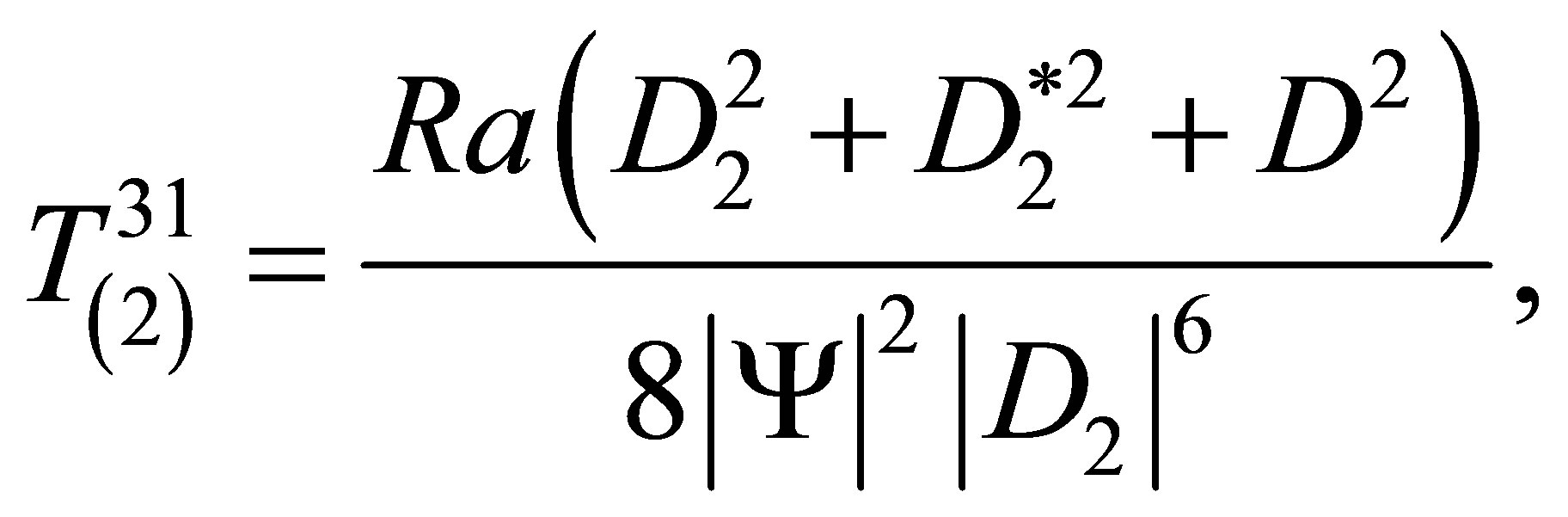
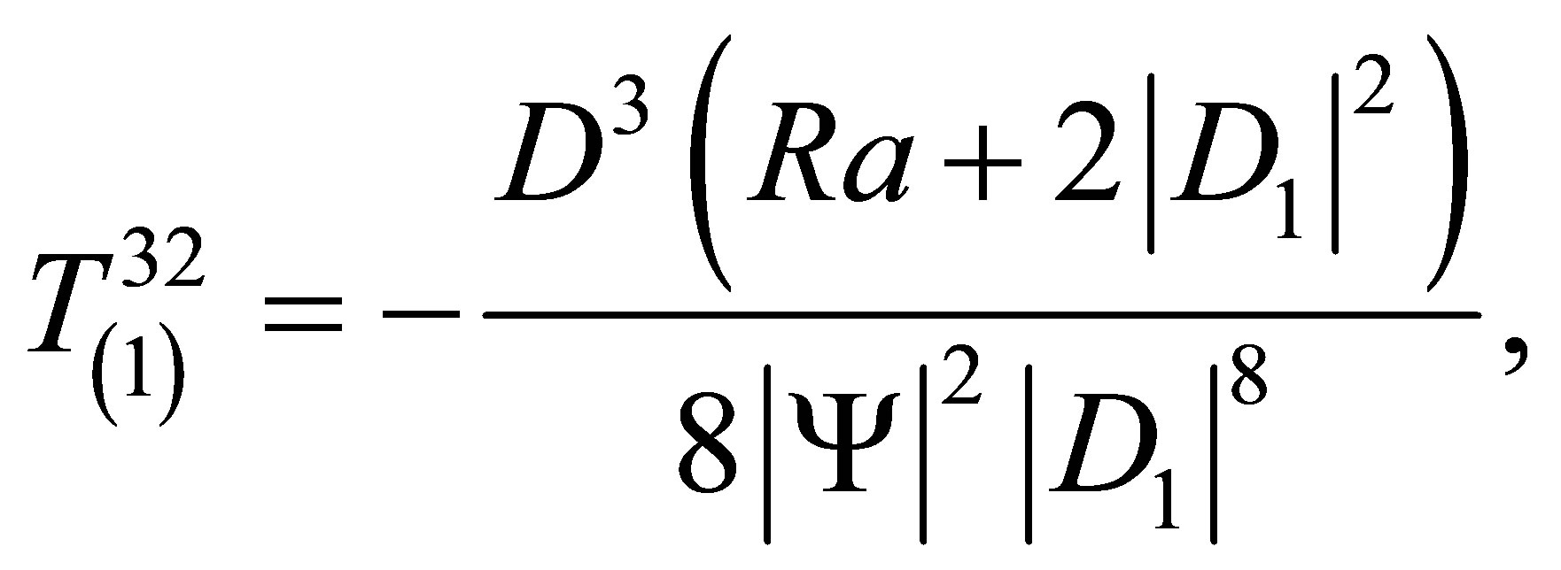
We can then express ,
,  ,
,  and
and :
:


where
5. Large Scale Instability
Let us write down in the explicit form the equations for nonlinear instability:
 (83)
(83)
 (84)
(84)
where the components ,
,  ,
,  and
and  of the Reynolds stress tensor are as defined in the previous section.
One can see that for small values of the variables  and
and , Equations (83) and (84) are reduced to linear equations and describe the linear stage of instability:
 (85)
(85)
 (86)
(86)
where the coeficients ,
,  ,
,  and
and  can be written as
 (87)
(87)
with
 (88)
(88)
 (89)
(89)
 (90)
(90)
 (91)
(91)
and
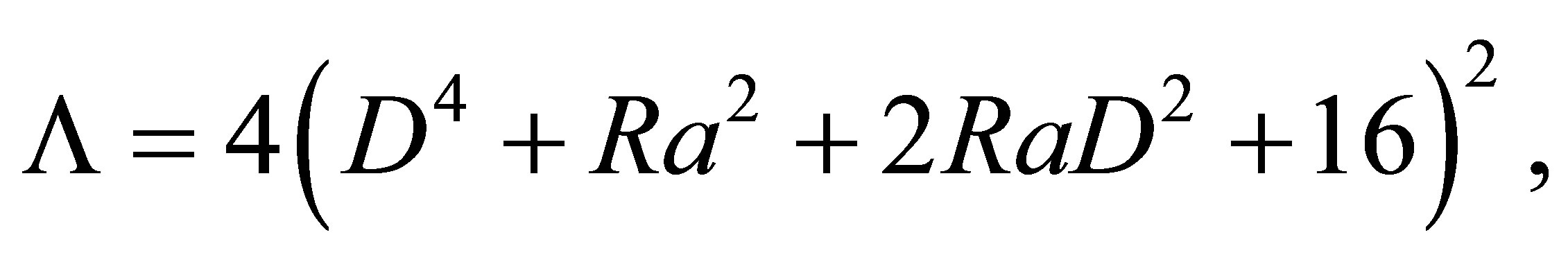 (92)
(92)
which are the explicit forms of the quite bulky coefficients. However, these coefficients can be expressed using the internal helicity  of the velocity field
 , calculated in Appendix B.
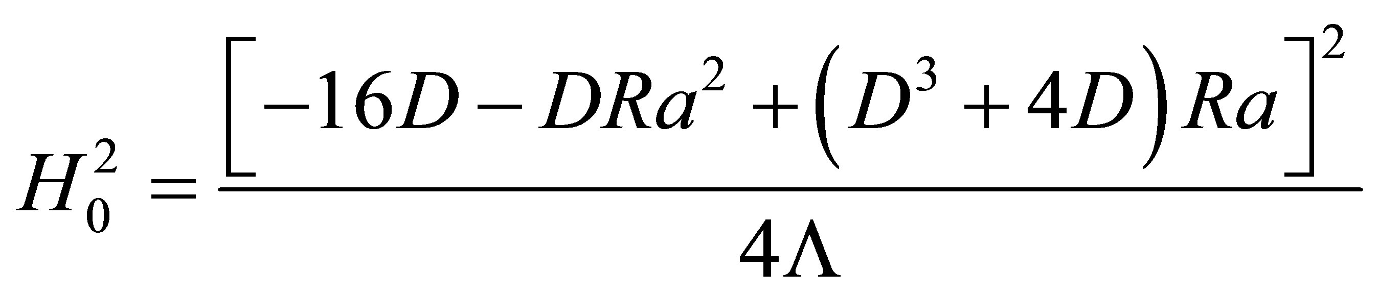 .
.
Therefore, we can write the constant coefficients  and
and  with respect to
 :
:
where .
.
Equations (85) and (86) can then be rewritten:
 (93)
(93)
 (94)
(94)
These formulas show that despite the zero helicity of the driving force, inside the system, an internal helicity is generated as a result of the joint impact of the Coriolis and buoyancy forces. This helicity plays an important role in the dynamics of the perturbations.
5.1. Unstable and Oscillatory Modes in the Case of Negligible Viscosity

In order to find instabilities, we choose the velocity  in the form:
 (95)
(95)
Injecting these solutions into (85), we obtain the simple system of equations:
 (96)
(96)
Evidently we get a quadratic equation for :
:
which allows us to obtain the dispersion equations for the different modes.
5.1.1. Dispersion Equation for the Unstable Mode
This equation is obtained by searching for solutions of (96) for which the discriminant is negative, namely, . We show Figures 1 and 2 representing the area (in gray) of the plane
  for which the discriminant is negative, this means that an instability can appear. Figure 1 shows the conditions for a negative temperature gradient and Figure 2, for a positive one.

Figure 1. Instability condition with negative temperature gradient.

Figure 2. Instability condition with positive temperature gradient.
Finally, we get

where
 (97)
(97)
(97) is the growth rate of the instability. We note that it is proportionnal to the square of the helicity.
5.1.2. Dispersion Equation for the Oscillatory Modes
This Equation is obtained by searching for solutions of (96) for which the discriminant is positive, namely, .
.
We obtain in this case two oscillatory modes,  and
and , which are, respectively, a slow and a fast mode:
 (98)
(98)
 (99)
(99)
It appears that both slow and fast oscillatory frequencies are proportional to the square of the helicity as well.
5.2. Unstable and Oscillatory Modes with Viscosity
In the same way as before, we get the system
 (100)
(100)
We can then get a new quadratic Equation for :
:

Dispersion Equation for the Unstable Mode
The discriminant of this Equation is the same as in the nonviscous case, so the dispersion equation for the unstable mode has the same condition, namely 
 , which leads to:

where
 (101)
(101)
It is to be noted that the growth rate  is maximal for
 , which can be considered as the characteristic scale of the generated vortex structures. Below is Figure 3 showing the evolution of
  with respect to the wave number
  for
for .
.
It can be noted that if the discrimant is positive, we get an oscillation with an exponentially decreasing amplitude.
With increasing amplitude, the instability becomes nonlinear and stabilizes. As a result, nonlinear vortex structures appear. The nonlinear stage of this instability and the results of numerical simulations will be presented in a future paper.
6. Conclusions and Discussion of the Results
In this paper, we showed that a large scale instability can appear in a rotating stratified fluid which is under the impact of a simple small scale external force (turbulence). The scale of this instability is much larger than the scale of the external force or turbulence. It is important to emphasize that, unlike previous papers about large scale instabilities, in the present paper, there are no special constraints imposed on the external force. It has a zero helicity and its parity needs not be violated; this means that this is a general force. Nevertheless, the small scale turbulence under the impact of the Coriolis force and the buoyancy force becomes helical. This helicity , finally, is responsible for the generation of large scale instabilities because the growth rate
  is proportional to
 . The instability itself is oscillating while its frequency
  and
and  have, in principle, the same order. This means that the instability in the general case is aperiodic. The frequency of both the stable and unstable oscillations is also proportional to
 . So we can say
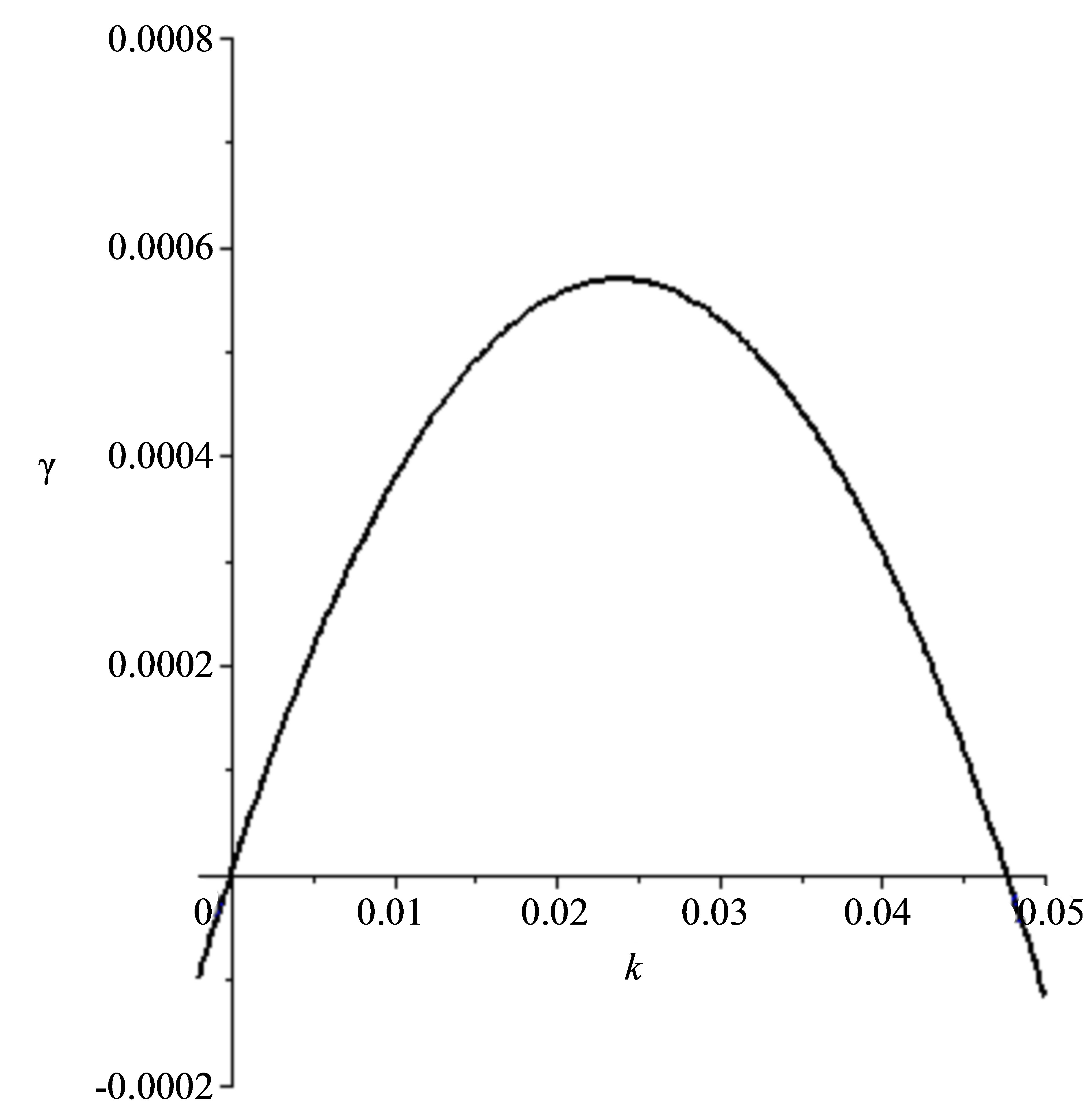
Figure 3. Evolution of the growth rate with respect to .
.
that the oscillation modes are inertial oscillations of the rotating fluid strongly modified by the helicity. There are two oscillating modes: one slow  and one fast
 . These oscillations decay when the viscosity is taken into account and in the case of instability, the maximal growth rate is reached at a characteristic scale of
 . Thereby this scale is typical for vortex structures like Beltrami’s runaways. In this paper, the theory of a large scale instability was constructed using the method of multi-scale developments, which was proposed in the work of Frisch, She and Sulem [11]. The nonlinear secular equations for the large scale instability were obtained in the third order of development on a small Reynolds number. In this paper, we studied in detail the linear stage of the instability and the conditions of its appearance. It is interesting to note that instability is possible in the case of both stable and unstable stratifications. Moreover, that neither the Rayleigh number nor the Taylor number are assumed to be either big or small: this means that these numbers are out of scheme parameters. That is the reason why we should state that
 , where
  is the critical Rayleigh number for the generation of convective instability. The unstable stratification is typical for atmosphere dynamics while the stable one is typical for ocean dynamics. We believe that the instability which was found in this paper could be applied to the issue of the generation of large scale vortices in the atmosphere and the ocean, and to some astrophysical problems as well.
Appendix
Calculation of the Reynolds Stress Tensor
In order to calculate the Reynolds stress, we begin with the general expression
 (102)
(102)
with
 (103)
(103)
and
 (104)
(104)
Hence,
 (105)
(105)
and  has a similar expression.
Taking into account that only the components  and
and  of the external force are nonzero, and after some factorizations, we can write the two contribution of the Reynolds stress tensor in the following form:
The same calculation for the contribution  gives us

Calculation of the Helicity
The driving force has no helicity, but the joint action of the external force, Coriolis force, and the buoyancy give the internal helicity.
The general helicity of the velocity field  is expressed by
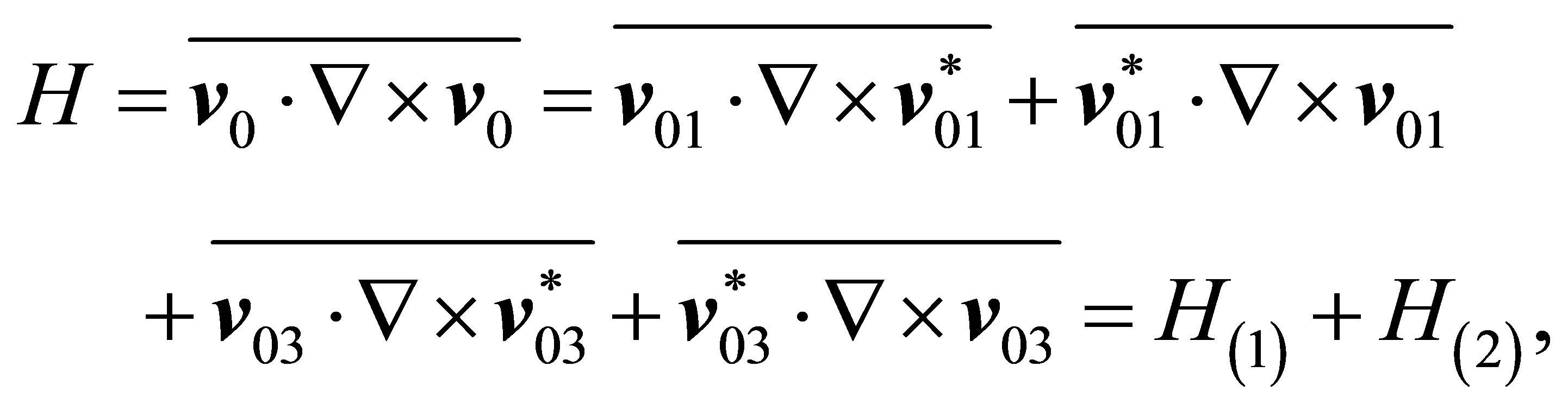 (106)
(106)
where we choose  and
and  such that

and
and in indicial notation:
We must calculate  with
with
 is calculated in the same way, by replacing
  with
with .
.
We finally obtain
After linearization:
where we recall that .
.
One can note that for small perturbations , the helicity approaches the constant:
which can be considered as the internal helicity of the field  when there are no perturbations.