Waiting Time Distribution of Demand Requiring Multiple Items under a Base Stock Policy ()
1. Introduction
It is important for production and inventory systems to attain the minimal inventory and shortage costs. In Zipkin [1] many inventory and production policies are discussed. As an inventory policy in production and inventory systems with stochastic demand, a base stock policy is important and well-known. Under this policy, the total number of work-in-process and finished items in the system retains constant. That is, when the demand arrives at the same amount of products, the demand requires are ordered at the same time, and if there are finished items enough to satisfy the demand, then it is satisfied, and otherwise it waits for the completion of processing items.
The production and inventory system with demand requiring multiple items under base stock policy has the following two types. First is the model in which the demand is decomposed to multiple units each of which corresponds to each item required, and each unit is satisfied immediately when this item is produced. This is the case that multiple demands arrive at the system at the same time. It is found when a retailer orders items on multiple customers and each customer is satisfied when the item on his order is produced. The second case is that each customer requires multiple items and orders them to the system. In this case, the customer is satisfied when all items she/he orders are produced. For example, if some products fail and repair parts are required, then multiple parts are needed for repair.
In the first case the waiting time for each unit has been analyzed. The arrival process is assumed to be a compound Poisson process, in which the interarrival time of demand forms Poisson process and the numbers of arrivals at the same time have the same probability function and they are mutually independent. In Feeney and Sherbrooke [2], the waiting time distribution of the demand is analyzed, and recently in Zhao [3] the network with multiple production and inventory systems is analyzed.
In the second model, Higa et al. [4] derive the waiting time distribution of demand when a probability mass function of items the demand requires is a geometric distribution, which is not practical in many situations. In the other model, Ko et al. [5] analyze an approximate lead time distribution in an assemble-to-order production system.
In this study, the waiting time distribution of demand, in the second model with a general distribution on the numbers of items the demand requires, is analytically derived. The expression of the MX/G/1 waiting time distribution with service time distribution in some class, which is discussed in Chandhiry and Gupta [6], and the probability distribution on the order unit corresponding to an item each unit of the demand requires, which is obtained in Zhao [3], are used in our analysis. The analytical method for deriving the waiting time distribution of demand is developed. Through numerical experiments properties of the waiting time distributions are discussed. It is used for finding the optimal number of base stocks, which is a minimal number of base stocks satisfying the condition that the fraction of demand who waits for items for period less than or equal to a predetermined time must be greater than a pre-specified value.
The organization is as follows. In Section 2, the model analyzed in this paper is described. In Section 3, the waiting time distribution for each demand is analyzed theoretically. In Section 4, the numerical analysis is given and Section 5 concludes the paper.
2. Model Description
2.1. Model
A production and inventory system is considered with a single product and demands for requiring multiple items. The number of items each demand requires is stochastic and has distribution pn = P(X = n), n = 1, 2,···, U, where U is its maximal size. The expectation is denoted by E[X]. The sizes of items which successive demands require are mutually independent, and demand arrivals form a Poisson process with rate λ. As a result, the arrival process on item requirements forms a compound Poisson process.
The system follows a base stock policy. Figure 1 illustrates the system. The number of base stock is denoted by s. When the demand arrives and requires multiple items, the system orders the same number of items for production. At the same time, if there are items enough for the demandto require, then it is fulfilled immediately, and it receives items and leaves the system. If it is not enough or the other demand waits for items, then it waits for all items which it will receive to be processed andplaced at the inventory. Note that the demand is fulfilled under a first come first served rule.
In the following, it is assumed that each demand consists of multiple units, each of which requires one finished item.Units are numbered 1, 2, ···, n when demand takes n order units, and unit 1 means the first unit of the demand, unit 2 means the second unit of the demand, and so on. The unit n is called the last unit.
When an order is received, a production process produces items. If there are multiple order units, each unit waits for production in a queue. The processing time is mutually independent and identically exponentially distributed with rate μ. Therefore, the units in the production
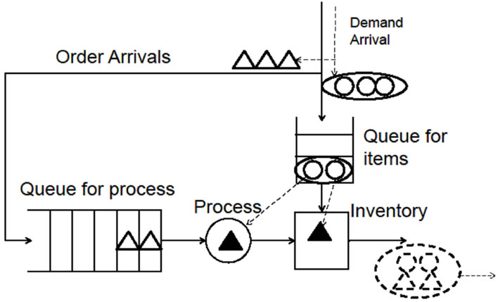
Figure 1. Production and inventory system under a base stock policy (s = 2).
process form an MX/M/1 process with arrival rate λ, the batch size distribution pn and exponential service rate μ. Here it is assumed that , which assures that the number of orders waiting for process is finite almost surely.
The objective of this paper is to analytically derive the waiting time distribution of demand in a steady state, that is, the time interval from the demand arrival epoch to the finishing epoch of process for all units satisfying this demand.
2.2. Waiting Time of Demand
The relations among waiting time of demand, interarrival time of demand and processing time of items are discussed. They are illustrated in Figure 2. Specific demand is fulfilled and departs the system when all units on the demand are satisfied. The waiting time of the demand is defined as the sojourn time of specific demand from its arrival to its departure when all units are fulfilled. We make attention to the last unit of the demand (which is painted in black in Figure 2). This order unit is satisfied when the processing of product corresponding to the s-th previous unit from this unit is completed, because the system is under base stock policy with base stock s.
The following notations are used:
W: the waiting time of specific demand in steady state,
 : the interarrival time from the (n − 1)st demand to the nth demand numbered backward from the specific demand (n = 1, 2, ···).
Xn: the batch size of units on the nth demand backward before the specific demand,
 : the processing time on the mth unit of the nth demand backward from the specific demand. (m = 1, 2, ···, U, n = 1, 2, ···).
Wq: the time interval from the arrival time of order, which includes the s-th previous unit from the last unit of the specific demand, to the start of processing on the first unit of this order.
Note that Wq depends only on the arrival process before this order arrival, and thus Wq and  are independent of {
 , i = 1, 2, ···, n}, and from the assumption of compound Poisson process, {
 , i = 1, 2, ···n} and

Figure 2. Relations among waiting time of demand, interarrival time of demand and processing time of items.
{Xi, i = 1, 2, ···, n} are also mutually independent.
3. Analysis of Waiting Time of Demand
The N(k)-th demand backward before the specific demand includes the order on the item which the k-th unit of the specific demand receives, and M(k) denote the marked number of this unit in the N(k)-th demand. From the total probability law, we have
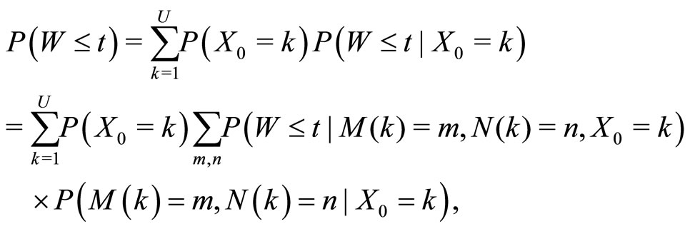 (1)
(1)
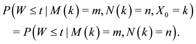
where X0 is the size of units of the specific demand. Since W is independent of X0 when M(k) and N(k) are given, it follows that
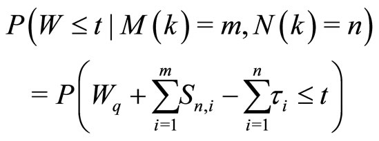
As shown in Figure 2, the waiting time of the specific demand W is equal to Wq, the waiting time of the corresponding order which includes the unit which processes the product of specific demand, plus the totalservice time on requirements in front of this unit, minus the interarrival time between the demand and this order. That is,
In the following, this distribution is analyzed theoretically.
3.1. MX/M/1 Waiting Time Distribution
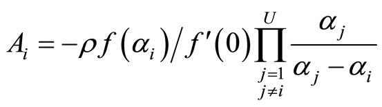
From the result on MX/M/1 queue waiting time distribution analyzed in Chandhiry and Gupta [6], in the model of this paper it is derived that
 for t>0where α1,···, αU denotethe U solutions except zero which satisfy the (U + 1)-st order equation
 , (2)
, (2)
and
 by letting
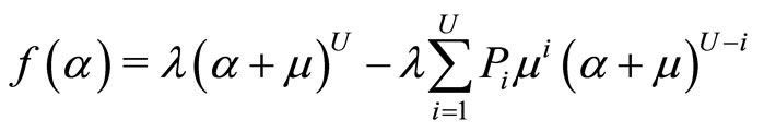 .
.
If this equation has z pairs of conjugate complex solutions and U-2z real solutions, then for some real constants  it is expressed that for t ≥ 0
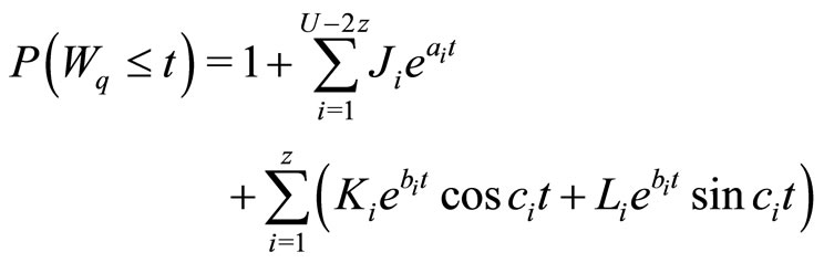 (3)
(3)
3.2. Analysis of Waiting Time Distribution
When n = 0, then  (1 ≤ m ≤ U) follows the Erlang distribution. Thus for t ≥ 0
In the following the case n ≥ 1 is considered. The value of  may be positive or negative.
1) When x ≥ 0, it can be obtained that after some calculations

where

This leads to the following density function.

where if n = 1 the first term on the right hand is zero.
2) When x<0, it follows that

Thus

where . From these equations, it follows that for n ≥ 1
where .
.
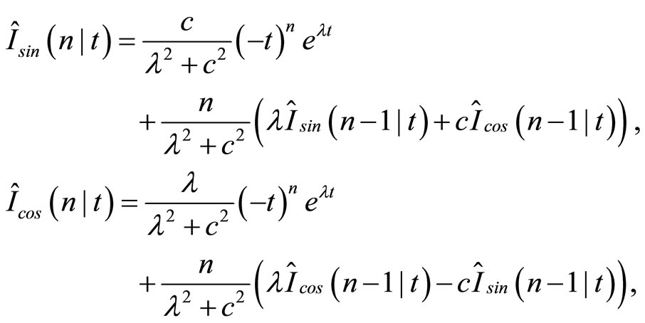
Note that by (3) this equation includes the following types of integrals:

and
These can be computed by the following recursive equations.

with
and in the same way
3.3. Probability on Position of the Corresponding Order and Unit
The probability on the position of the corresponding order and unit satisfying the last unit of the specific demand can be obtained by Zhao [3], which is given by
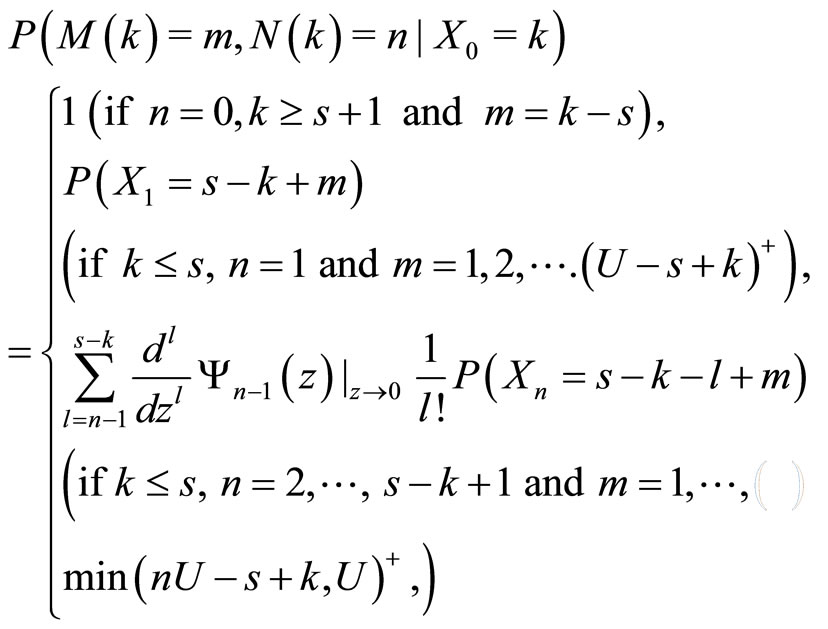
where  is a probability generating function of the k-fold convolution of p(n).
From the above equations derived in Sections 3.2 to 3.3, the waiting time distribution of the demand in the steady state can be obtained by Equation (1).
4. Examples
In this section waiting times and optimal base stocks are illustrated through examples. It is set as  and the maximal size is U = 3 through examples.
Example 1 P1 = 0.3, P2 = 0.4, P3 = 0.3, E[X] = 2, λ = 0.4, ρ = 0.8;
Example 2 P1 = 0.1, P2 = 0.8, P3 = 0.1, E[X] = 2, λ = 0.4, ρ = 0.8;
Example 3 P1 = 0.3, P2 = 0.4, P3 = 0.3, E[X] = 2, λ = 0.45, ρ = 0.9;
Example 4 P1 = 0.1, P2 = 0.3, P3 = 0.6, E[X] = 2.5, λ = 0.32, ρ = 0.8.
The waiting time distributions of demand are derived by the analytical method obtained in Section 3 and Wolfram Mathematica 8.0. For example, in example 1with base stock s = 1, the waiting time distribution of demand is derived as
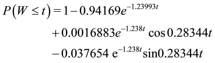 where there are other terms such as e−t, te−t, and t2e−t on the right hand side but they are removed because their coefficients are negligible small as their absolute values are less than 10−10. In example 1, the solutions of (2) except zero are −1.23800 + 0.28344i, −1.23800 − 0.28344i and −1.23993, where i is a purely imaginary number. In example 2, all solutions are real numbers, −1.54098, −1.14098 and −0.14098.
Tables 1 and 2 show the probabilities that the demand has no waiting time and those that the waiting time of demand is no more than 10, under base stock policies with base stocks 1 to 5 in examples 1 to 4, respectively.
First the result in Example 1 is compared with that in Example 2, which has the same expected number of items required by each demand, and the same arrival rate, but different variances on the numbers of required items. As shown in Table 2, if the variance is smaller, then the probability that waiting time of demand is no more than 10 is smaller. This effect is usually seen in inventory and queueing processes that more variance of components in the process leads to the greater waiting time. As Table 1 shows, however, when s = 1 the probability that demand has no waiting time in Example 1 is greater than that in Example 2. The reason is as follows. When s = 1, if the unit size of the demand is 2 or 3 then the last unit of demand is fulfilled by producing the item ordered by the former unit of the same order, and so the demand requiring for multiple items waits for completion of processing almost surely. If the unit size of the demand is 1, then the demand is satisfied by producing the item ordered by some unit of the former demand, so there is a possibility that the demand with one unit has no waiting time. Example 1 has the greater probability of the demand with one unit than Example 2, and so the probability that the demand has no waiting time is greater in Example 1.
For Example 3, which has the greater arrival rate, the above probabilities are much smaller than those in Example 1. Compared with Example 1, Example 4, which has the same intensity and more expected items required, leads to more waiting time and the above probabilities become small. This is because the interarrival times on the orders have more variances, and the process on the number of finished items in inventory alsoluctuates more. Thus Example 4 has more chances that when the demand arrives there is no item in inventory and it waits for finished items.
Table 3 shows the probabilities that demand with each size of units has waiting time no more than 10 for s = 1, 2, 3 in Example 1. When the size is greater, the probability is smaller, because the demand with more units has to wait for completion of the item ordered by recent demand or the latter unit, compared with the demand with one unit. Note that the probabilities for pairs (s, k) are the same when the value of s-k is the same. It is because when s-k is the same, the last unit of the specified de-
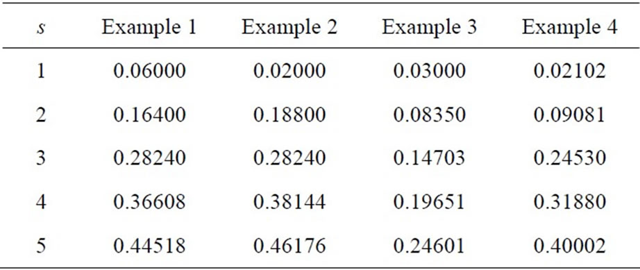
Table 1. Probabilities that demand has no waiting time.
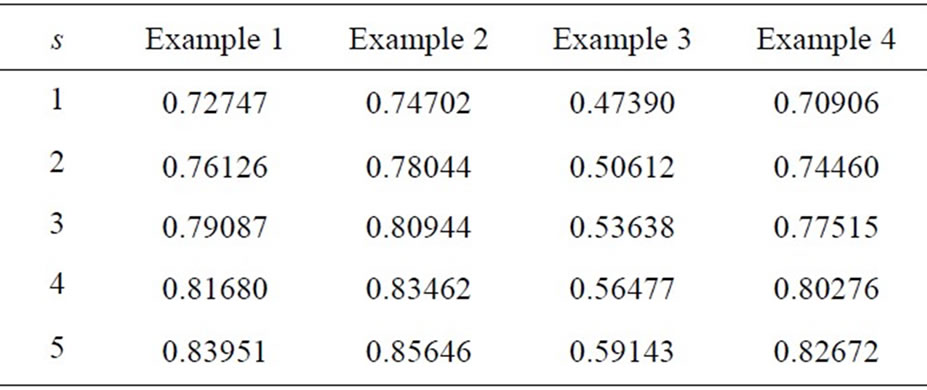
Table 2. Probabilities that demand has waiting time no more than 10.

Table 3. Probabilities that demand which has 1/2/3 units has waiting time no more than 10.
mand with k units requires the same item under the base stock policy with s base stocks. For example, demand with 2 units requires the item ordered by the last unit of its previous demand under s = 2, which is the one that demand with 3 units requires under s = 3.
Table 4 shows the probabilities that the waiting times are no more than t for t = 0, 5, 10, 15, 20 in cases s = 1 to 5 of Example 1. As s increases, the probabilities also increase, but the differences are the smaller when t is greater.