Extended Generalized Riccati Equation Mapping for Thermal Traveling-Wave Distribution in Biological Tissues through a Bio-Heat Transfer Model with Linear/Quadratic Temperature-Dependent Blood Perfusion ()
1. Introduction
Heat transfer in biological systems is relevant in many diagnostic and therapeutic applications involving either decrease or increase of temperature and often requires precise monitoring of the spatial distribution of thermal histories that are produced during a treatment protocol [1-9]. Since the pioneering work by Henriques and Moritz [10] and by Pennes [11] on heat transfer in biological system, the problem of heat transfer in biological systems has received renewed attention and has been the focus of considerable research [12-16]. The investigation of such heat transfer problems requires the evaluation of spatiotemporal distributions of temperature and has been traditionally addressed using the Pennes model which is originally designed for predicting temperature fields in the human forearm [10,11]. Pennes model of the heat transfer in biological systems accounts for the ability of tissue to remove heat by both passive conduction (diffusion)
and perfusion of tissue by blood. Here, perfusion is defined as the nonvectorial volumetric blood flow per tissue volume in a region that contains sufficient capillaries that an average flow description is considered reasonable.
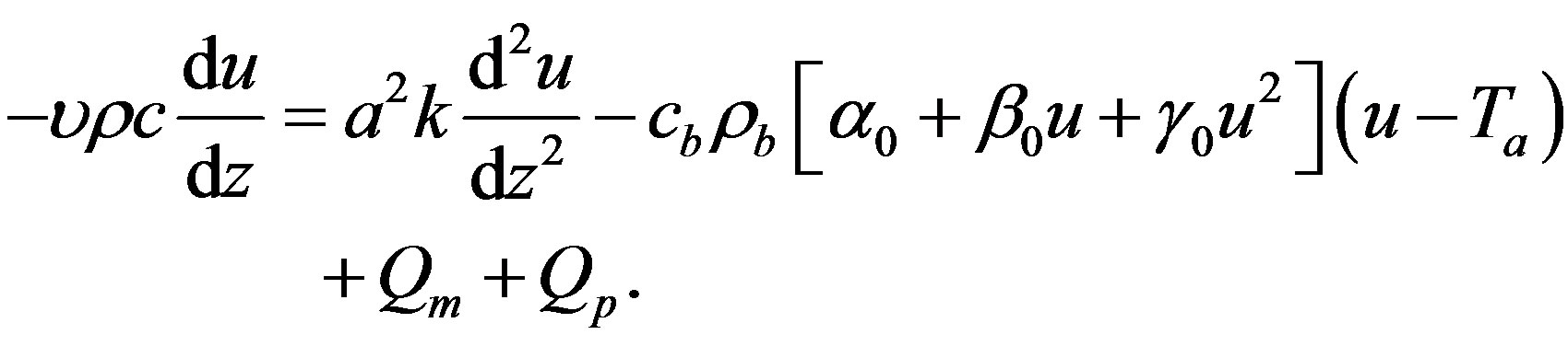
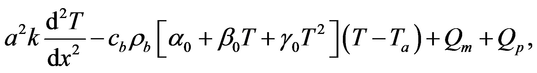
After performing a series of experiments which measured temperatures of human forearms, Pennes derived a thermal energy conservation equation called the “bioheat transfer” (BHT) equation or the traditional BHT equation. The generalized one-dimensional Pennes BHT equation can be written in the following form [17-21]
 (1.1)
(1.1)
where  is the local tissue temperature (temperature elevation);
  and
and  denote the time and the distance from the skin surface to the body core, respectively;
  is the arterial blood temperature (ambient temperature of perfusing blood);
  is specific heat of blood;
  is the density of blood;
  is the blood perfusion;
  is the tissue specific heat;
  is the tissue density;
  is the tissue thermal conductivity;
  is the regional heat delivered by the source;
  is the heat generation in the body, that is, the heat generated by the normal processes in the body, which is usually very small compared to the external power deposition term
  [22]. When the metabolic heat generation rate (
 where
where  is the total heat) is positive, body temperature will rise and when
  is negative, it will go down [23]; we remember that the total heat
  transported across a flat surface of area
  and thickness
  is related to the temperature gradient across the surface
  and the thermal conductivity of the material:
 . Equation (1.1) describes the influence of blood flow on the temperature distribution in the tissue in terms of volumetrically distributed heat sinks or sources.
The second term  in the right hand side (r.h.s.) of Equation (1.1) models the perfusion heat loss and can be the dominant form of energy removal when considering heating processes. Vascular tissues generally experience increased perfusion as temperature increases. The above term is always considered in cases of tissues with a high degree of perfusion, such as liver. Regarding cardiac ablation, the perfusion heat loss is incorporated in some models, but is generally ignored since its effect is negligible [24]. In general,
  is assumed to be uniform throughout the tissue. However, its value may increase with heating time because of vasodilatation and capillary recruitment.
Spatially distributed heating occurs in skin exposed to penetrating, dissipative radiation such as microwave, ultrasound, and laser light [25-27]. These heating methods often involve an exponentially decaying power transmission accompanied by reflection at the interface of regions with different electrical properties. For a uniform plane wave incident normally upon the skin surface, with a layer of air included to model the reflection at the skin/air interface, the average absorbed power density
 is given by:
  where
where  and
and  are the total electric field in the tissue and the electric conductivity, respectively.
Prediction of temperature in tissue models generally assumes a constant-rate (temperature independent) blood perfusion within each tissue and has long been carried out by both analytical and numerical methods based on Equation (1.1). In this case, the temperature rise can be easily predicted by traditional analytical methods based on Equation (1.1) and given boundary conditions, which can either be solved analytically for simple geometries [28,29] or by finite element method or finite-difference method for more realistic, complicated tissue geometry [30,31].
Several experiments have shown that the response of vasculature in tissues to heat stress is strongly temperature-dependent [32]. Obviously, models which include temperature-dependent increases in perfusion are more difficult to solve. The case of a linear temperature-dependence has been described combining analytical simulations [9,33,34]. Lang et al. [33] described an optimization process specially designed for regional hyperthermia of deep-seated tumors in order to achieve desired steadystate temperature distributions. To predict the temperature, they applied a nonlinear three-dimensional heat transfer model based on temperature-dependent blood perfusion. Using linearly implicit methods in time and adaptive multilevel finite elements in space, they were able to integrate efficiently the instationary nonlinear heat Equation with high accuracy. Temperature distributions for two individual patients calculated on coarse and fine spatial grids were compared. Most recently, Partridge et al. [35] presented an inverse analysis procedure based on a coupled numerical formulation first to identify the coefficients of linear and quadratic variations of blood perfusion, and then to investigate temperature distribution at the skin surface for tumor perfusion. Their procedure has the advantage of not requiring the calculation of derivatives or sensitivities, or an initial estimate of these values.
We assume in this work a linear and a quadratic temperature-dependent blood similar to the expression identified respectively by Gowrishankar et al. [36] and Partridge et al. [35]:
 (1.2)
(1.2)
where 

 , and
, and
 are three real parameters.
represents the baseline perfusion while  and
and  are respectively the linear and quadratic coefficients of temperature dependence. The unit employed for coefficient
 and
and  is such that
  represents mass flow rate of blood per unit volume of tissue. Based on the Pennes BHT Equation (1.1) with the blood perfusion (1.2), we aim in the present work to analytically investigate thermal traveling-wave distribution in biological tissues. We consider only the case of constant spatial heating, that is, the case when
  .
.
In our knowledge, there has not yet being reported a scientific work that treats thermal traveling-wave distribution in biological tissues by means of Riccati Equation
 (1.3)
(1.3)
In Equation (1.3),  and
and  are two real functions of
 . The Riccati Equation, though a nonlinear Equation, is characterized by the fact of possessing a superposition formula, as it is the case for all linear equations. Moreover, Riccati equation can be linearized; indeed, we can use the Cole-Hopf transformation [37,38] to reduce it to a linear Schrödinger spectral problem. Riccati Equation (1.3) appears in many fields of applied mathematics, in many instances when we can find exact solutions of nonlinear partial differential equations. In mathematical literatures, Riccati Equation (1.3) is known as the only first order nonlinear ordinary differential equation which has no movable singularity, i.e., which possesses the Painlevé property [39,40]. As it was shown by Lie et al. [41], Riccati Equation (1.3) admits a (nonlinear) superposition formula
 (1.4)
(1.4)
that is, if 
 and
and  are three solutions of Equation (1.3), and
  will also be a solution of Equation (1.3), with
  being a constant parameter. The nonlinear superposition Formula (1.4) allows us to build a denumerable set of solutions of Riccati Equation (1.3), as soon as three of its solutions are found.
The aim of the present work is to apply Riccati Equation (1.3) to analytically investigate thermal traveling-wave distribution in biological tissues through the BHT model (1.1) with the temperature-dependent blood perfusion (1.2). The rest of the paper is organized as follows. In Section 2, we explore the solutions of Riccati Equation (1.3) in the special case of constant coefficients  and
and  In Section 3, we apply the generalized Riccati equation mapping method [42] to find solutions to Equation (1.1) with perfusion (1.2). Here, we distinguish the initial processus (temperature at each distance
  from the skin surface to the body core at time
 ), instantaneous temperature distribution of biological tissues (temperature at each distance
  from the skin surface to the body core at a given time
 ), and the steady-state temperature distribution (the temperature of each point
  of the biological tissue is constant with respect with time). The results are discussed in Section 4 and summarized in Section 5.
2. Solutions of Riccati Equation (1.3) in the Special Case of Constant Coefficients  and
and 
In this section, we explore the possible solutions of Riccati Equation (1.3) in the special case of constant coefficients  and
and  Let us consider Riccati equation
 (1.5)
(1.5)
where 
 and
and  are three real parameters with
 . One easily verify that transformation
  reduces Equation (1.5) into the second order linear ordinary differential equation (ODE) with constant coefficients
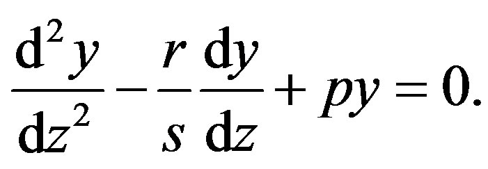 (1.6)
(1.6)
It is also well-known that the transformation  reduces the Riccati Equation (1.5) into the the below first order ODE as soon as
  is a particular solution of (1.5)
 (1.7)
(1.7)
Integrating Equations (1.6) and (1.7) yields
 (1.8)
(1.8)
 (1.9)
(1.9)
respectively, where  and
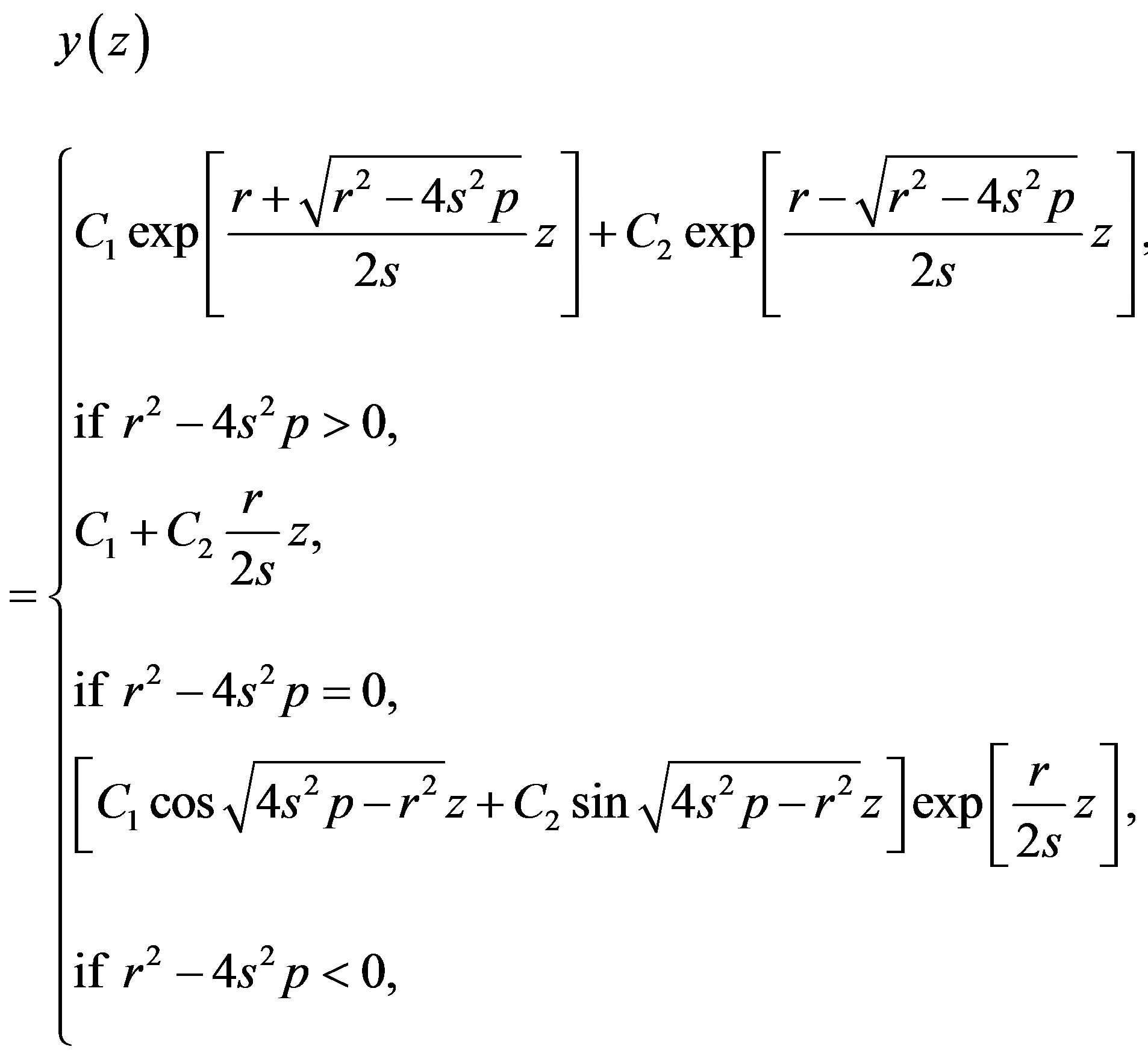
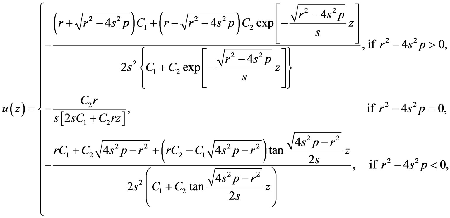
and  are two arbitrary real constants. Expression (1.8) gives the following general solution of Riccati Equation (1.5)
 (1.10)
while expression (1.9) gives the following general solution of Riccati Equation (1.5)
 (1.11)
Really speaking, solution (1.10) contains only one free parameter, namely, 
3. Thermal Traveling-Wave Distribution in Living Tissues
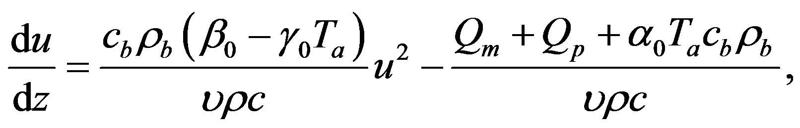
With the help of Riccati equation, we investigate in this section the thermal traveling-wave distribution in biological tissues through the BHT Equation (1.1) with the temperature-dependent blood perfusion (1.2). In other words, we present in this section the application of the Riccati equation to find analytical traveling-wave solutions of equation
 (1.12)
with constant . We start by transforming Equation (1.12) into a nonlinear ordinary differential equation by introducing the variable
  given by
 (1.13)
where  and
and  are two arbitrary constants (
 is the wave velocity). Inserting ansatz (1.13) into Equation (1.12) yields
 (1.14)
We first apply the generalized Riccati equation mapping method, and then a simple coupling method to find analytical solutions of Equation (1.14).
3.1. Generalized Riccati Equation Mapping Method for Temperature Distribution in Biological Tissues
The generalized Riccati equation mapping method assumes that Equation (1.12) admits solutions that can be expressed as a polynomial of degree  in
in 
 (1.15)
where  are real constants to be determined and
  is solution of the Riccati Equation (1.5). The first step in this method consists of determining
 . To determine
 , we consider the homogenous balance between the highest order derivative and the highest order nonlinear terms. After finding
 , one substitutes Equation (1.15) into Equation (1.14) and use the fact that
  is a solution of Equation (1.5). Then, one collects all terms with the same order of
  and
and  If the coefficients of
  and
and  vanish separately, one will obtain a system of algebraic equations in


 and
and  that physical solutions can be found with the help of Mathematica (here, physical solution means solutions of the algebraic system that define physical solutions of Equation (1.1) with perfusion (1.2)). Finally, one uses the solutions of Riccati Equation (1.5) found in the previous section, and goes back in original variables
  and
and  through ansatz (1.13) to obtain travelling wave solution of Equation (1.12).
Let us now turn to the concrete case of Equation (1.5). We start by inserting Equation (1.15) into Equation (1.14). Using the fact that  is a solution of Equation (1.5) and balancing the highest order of derivative term and nonlinear term, we get that
  for a quadratic blood perfusion, and
  for a linear blood perfusion. So that Equations (1.15) and (1.5) give
 (1.16a)
 (1.16b)
for quadratic and linear blood perfusion, respectively. By combining solution (1.10) of Riccati equation and expression (1.16a) and going back to original coordinates ,
,  , and
, and  one easily sees that The steady-state analytical solution to the bio-heat Equation (1.1) with blood perfusion (1.2.) differs with a spatially distributed uniform sink given in Ref. [43].
Case of a quadratic temperature-dependent blood perfusion
Let us start with the case of a quadratic blood perfusion, that is, when . Then Equation (1.14) admits solutions of form (1.16a). Inserting Equation (1.16a) into Equation (1.14) and imposing to the coefficients of
  and
and  to vanish separately, we obtain, after the compatibility requirement, the algebraic system (see (1.17) below)
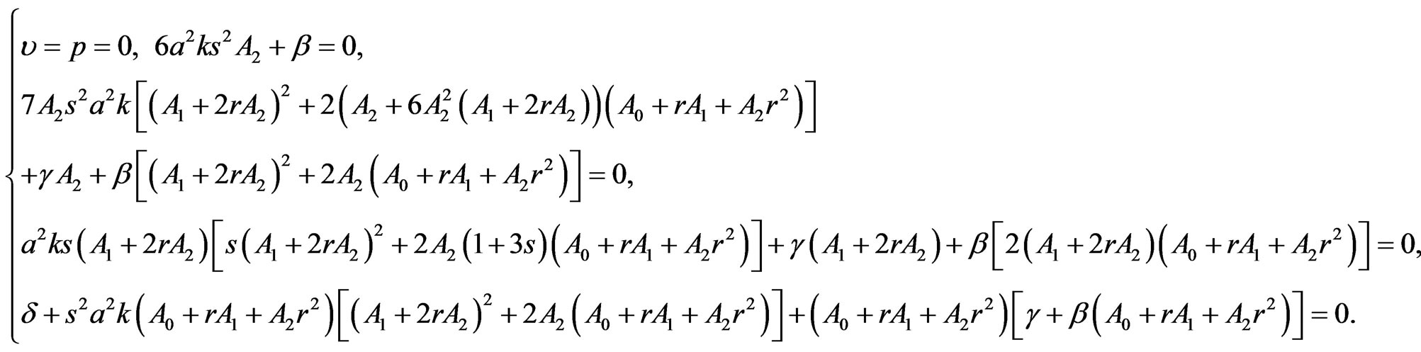
Here,

 (1.17)
It should be noted that condition  corresponds to either the initial temperature distribution or the steadystate temperature distribution. Indeed, the initial temperature distribution and the steady-state temperature distribution in biological tissues is obtained by integrating the ordinary differential equations
 (1.18)
 (1.19)
respectively. Substituting ansatz (1.13) with  into Eqs. (1.18) and (1.19), we obtain Equation (1.14) in which
  is replaced by 0. It is important to point out that the term
  is absent in Equation (1.18). Indeed, prior to heating process, there is not any heating source. Thus, for the initial temperature distribution and the steady-state temperature distribution, we will work with
  and
and  with
with  any real constant. We notice that in the case of absence of heating sources, the initial temperature coincides with the steady-state temperature fields.
Case of a linear temperature-dependent blood perfusion
Here, we consider the case of a linear blood perfusion, that is, when  and
and . As it is shown above, Equation (1.14) admits solutions of form (1.17). Inserting Equation (1.17) into Equation (1.14) and imposing to the coefficients of
  and
and  to vanish separately, we obtain, after the compatibility requirement, the algebraic system (see (1.20) below)
 (1.20)
Here,

Condition  means the generalized Riccati equation mapping method in the case of linear blood perfusion can be applied just for the initial temperature distribution and the steady-state temperature distribution.
3.2. Coupling Method for Thermal Traveling-Wave Distribution in Biological Tissues
In this section, we split Equation (1.14) into two ordinary differential equations which lead to a Riccati equation that will help us to find analytical solutions.
It is obvious that  will satisfy Equation (1.14) as soon as it verifies the following two equations
 (1.21a)
 (1.21b)
One easily verifies that any solution  of Equation (1.21a) will satisfy equation
 (1.22)
Therefore,  will satisfy Equation (1.21b) if and only, if Equation (1.21b) coincides with Equation (1.22), that is, if and only, if
  and
and
 (1.23)
Thus, if blood perfusion parameters 
 and
and  and the wave velocity
  satisfy condition (1.23), then any solution of Equation (1.21a) will be solution of Equation (1.14). Henceforth, we will focus ourselves on Equation (1.12a). When
  Equation (1.21a) coincides with Riccati Equation (1.5) with
 ,
,
 and
and 
Under condition  we obtain from particular and the general solutions of Equation (1.21a) the following solutions of Equation (1.1) with perfusion Equation (1.2)
 (1.24)
and
 (1.25)
respectively. Here,  and
and 
is an arbitrary real constant.
4. Results and Discussion
In this section, we use the analytical solutions found in the previous section to discuss thermal traveling-wave distribution in biological tissues.
In the following calculations, the typical tissue properties are applied as given in [20]: 


 for the healthy tissue and
  for the tumor. In our simulations, the skin surface and the body core are assumed to be defined at
  and
and , respectively. As it is shown by several investigators [44,45], the interior tissue temperature usually tends to a constant within a short distance such as 2 - 3 cm. Therefore we will choose
  in our simulations. Following Partridge et al. [35], we will use for the temperature-dependent blood perfusion (1.2), the coefficients
 (1.26)
where for tumour  takes values up to 7,
  takes values up to 1.9, and
  takes values up to 0.07. In the case of linear blood perfusion, i.e., when
 , we will take
  and
and  so that
  and
and  coincide with the coefficients of linear blood perfusion used in Ref. [36]. Because the variation of the constant spatial heating
  can only affect the temperature magnitude at a given depth
  we will, without loss of generality, consider in all our simulations that
  so that the initial temperature field for the basal state of biological bodies will coincide with the steady-state temperature fields.
We start our analysis with the case of linear temperature-dependent blood perfusion. Figure shows the initial/steady-state temperature distribution obtained in the case of linear temperature-dependent blood perfusion with the same baseline perfusion  and the linear perfusion coefficient
 , respectively. The physical solutions of system (1.20) used for this figure are showed in Table 1. As one can see from Table 1, the physical solutions contain two parameters,
  and
and . These two parameters can be defined in a concrete problem of heat transfer, for example, when the boundary conditions are given. For plots of Figure 1, we

Table 1. Solutions of system (1.20) obtained for the same baseline perfusion α0 and different linear coefficient β0.

Figure 1. (Color online) Initial/steady-state temperature-dependent perfusion distributions for different linear coefficient of temperature dependence in the case of linear temperature-dependent blood perfusion. The perfusion level was dependent on local temperature with the same baseline perfusion α0 = 0.1 and a linear coefficient of temperature dependence shown in inset. Top left: Effect of linear coefficient of temperature dependence on temperature distribution; here, we have used (C1, C2) = (0.01, 2) (see Equations (1.4)). Top and bottom right, bottom left: Spatial temperature distribution for different  and different (C1, C2) appearing in Equations (1.4) and (1.10), respectively; the same values of (C1, C2) and
 , shown in the bottom right plots have been used. The dashed and dotted curves show the temperature distribution obtained with the help of the nonlinear superposition (1.4).
have used  and
and . The 3 cm long tissue has being used. The top left plot shows the spatial distribution of temperature for different values of perfusion
  As expected, decreased perfusion causes a decline in local temperature. Each of other three figures shows for the same
  temperature distribution obtained for different parameters
  and
and  appearing in Equation (1.10) and different parameter
  of nonlinear superposition (1.4). The dashed and dotted curves show the temperature distribution obtained with the help of the nonlinear superposition (1.4); here, we have used three different
  to form the solutions for the superposition. As one can easily see from these three plots, different parameters
  give the same temperature at surface of the skin and at the body core. The top right and bottom left and right plots show that one may use the superposition parameter
  to manage (increase or decrease) temperature of the biological tissues.
Let us discuss the case of a quadratic temperaturedependent blood perfusion. We will focus our attention on the case  and
and , that is, the case of thermal traveling-wave distribution. We will investigate the effect of linear and quadratic coefficients of temperature dependence on temperature distribution, and then, show how one may used the parameter of the nonlinear superposition formula of Riccati equation to control the temperature in time and space.
Figure 2 shows the effect of the quadratic coefficient of temperature dependence on temperature distribution. For this figure, we have used the perfusion coefficients (1.26) with 
 The 3 cm long tissue has being used. For these values of
 and
and  physical solutions of system (1.17) are given in Table 2. For these physical


Figure 2. (Color online) Temporal and spatial temperature-dependent perfusion distributions: Effect of the quadratic coefficient of temperature dependence on temperature distribution. The left and right plots respectively show the temporal and spatial temperature distribution at different distance x from skin surface and at different time t. Plots (a), (b), and (c) show the temperature distribution at skin surface, at distance x = 0.015 m, and at the body core, respectively. Plots (d), (e), and (f) show the initial temperature distribution, the temperature distribution at time t = 10000 s, and the steady-state temperature distribution, respectively. For all these plots, we have used solution (1.4)) with (C1, C2) = (1, 1). Here, we have used p1 = 3, p2 = 0.5, and different p3 shown in plot (a) (see Equation (1.26)). We have used a = 0.20000000000000004, υ = −2.2704766042804436 × 10⁻⁷, A0 = −47.48257513976442, and r = 847.8483254334188 for p3 = 0.01; a = 0.28284271247461906, υ = −1.2284805279005027 × 10⁻⁶, A0 = −33.31293218373712, and r = 705.3092927447257 for p3 = 0.02; and a = 0.3464101615137755, υ = −1.9254281349374016 × 10⁻⁶, A0 = −27.89371450273014, and r = 650.6425537226606 for p3 = 0.03. Other parameters used for the realization of these plots are given in the text.

Table 2. Solutions of system (1.17) obtained for the same parameters p1 and p2 and different parameter p3: (a) (p1, p2, p3) = (3, 0.5, 0.01); (b) (p1, p2, p3) = (3, 0.5, 0.02); (c) (p1, p2, p3) = (3, 0.5, 0.01)
solutions,  and
and  appear as free parameters and can be particularized with the help of additional condition of the bio-heat transfer problem such as boundary conditions. For all plots of Figure 2, we have used
  and
and .
.
The left and right plots of Figure 2 respectively show the temporal and the spatial distribution of temperature at different distance  from the skin surface and at different time
  for different values of
  (i.e., for different values of the quadratic coefficient of temperature dependence of blood perfusion). As expected, increased perfusion causes a decline in local temperature. As it is seen from the left plots, the temperature of the tissue at each distance x from the skin surface decreases and approaches the steady-state temperature. It is also seen that with smallest
  the tissue temperature will quickly reach a steady state. As seen in right plots, tissue temperature decreases as one goes from the skin surface to body core.
To investigate the effect of linear coefficient of temperature dependence of the blood perfusion on temperature distribution, we fix  and
and  and vary
  as follows:
 . For these values of
  and
and  and
and  physical solutions of system (1.17) are shown if Table 3. This table shows two free parameters,
  and
and  which can be determined by using additional condition imposed on Equation (1.1) with potential (1.2).
Figure 3 shows the temporal (left plots) and the spatial (right plots) temperature distribution for a 3 cm long tissue. The plots of this figure have been generated with the help of Riccati solution (1.10). As solutions of system (1.17), we have used data from the first row of (a), (b), and (c) in Table 3, with  and
and . As constants of solution (1.10), we have used
  and
and  As seen in plots (a) obtained with
 , increased perfusion causes a decline in the temperature of skin surface. Plots (b) and (c) show that inside the tissue (when
 ), for a short period of heating, decreased perfusion causes a decline in local temperature. As one tends to the steady-state, higher perfusion gives lower local temperature. From plots (d) and (f) which respectively show the initial temperature distribution and the steady-state temperature fields, it is seen that increased perfusion causes an increase in the initial and steady-state local temperature of tissue.
Dashed and dotted curves of Figure 4 show the temperature distribution obtained with the help of nonlinear superposition formula (1.4) of Riccati equation. Other three curves of this figure show the temperature distribution obtained with the use of solution (1.10) after particularizing parameters  and
and ; we have used the same parameter
  and three different C1 = 17, 20, 23. To generate the solutions of the superposition, we have used
 and
and  and the following solution of system (1.17): α = 0.5291502622129182, υ = 0.00012855305358758568, A0 = 100.49771736484482, r = −634.2109797960809, A1 = 0.1,
 and s = 4. Plots (a) and (b) show respectively the temperature of skin surface and body core as function of time
 . Plots (c) and (d) depict the temperature curves as function of skin depth
  at time
  and time
  The four plots of Figure 4 show that one can easily readjust (increase or decrease) the temperature of the biological tissues, just by varying parameter
  of the nonlinear superposition formula (1.4) of Riccati equation.
Let us now validate solutions (1.24) and (1.25). This solution presents some restriction on blood perfusion (1.2). Indeed, 
 and
and  appearing in Equation (1.26) must satisfy the second equality in Equation (1.23). With this restriction, it is not possible to separately
Table 3. Solutions of system (1.17) obtained for the same parameters p1 and p3 and different linear parameter p2: (a) (p1, p2, p3) = (7, 1, 0.07); (b) (p1, p2, p3) = (7, 1.2, 0.07); (c) (p1, p2, p3) = (7, 1.4, 0.07).


Figure 3. (Color online) Temporal and spatial temperature-dependent perfusion distributions: Effect of the linear coefficient of temperature dependence on temperature distribution. The left and right plots respectively show the temporal and spatial temperature distribution at different distance x from skin surface and at different time t. Plots (a), (b), and (c) show the temperature distribution at skin surface, at distance x = 0.015 m, and at the body core, respectively. Plots (d), (e), and (f) show the initial temperature distribution, the temperature distribution at time t = 100 s, and the steady-state temperature distribution, respectively. For all these plots, we have used solution (1.4)) with (C1, C2) = (−17, 0.2). Here, we have used p1 = 7, p3 = 0.07, and different p2 shown in plot (a) (see Equation (1.26)). We have used a = 0.5291502622129182, υ = 0.00012855305358758568, A0 = 100.49771736484482, and r = −634.2109797960809 for p2 = 1; a = 0.5291502622129182, υ = 0.00013226855259313876, A0 = 102.1353600675383, and r = −650.6257480827784 for p2 = 1.2; and a = 0.5291502622129182, υ = 0.00013594278617606382, A0 = 103.73333731695307, and r = −666.6402113289303 for p2 = 1.4. Other parameters used for the realization of these plots are given in the text.

Figure 5. (Color online) Thermal traveling-wave distribution via either analytical solution (1.24) or (1.25).(a), (b), (c): Temporal temperature distribution at different skin depths x = 0.009 m, 0.021 m, 0.03 m, respectively. (d), (e), (f): Temperature distribution as a function of skin depth at different times t = 0 s, 500 s, 8000 s, respectively. The perfusion level was dependent on local temperature with the same baseline perfusion α0 = 5 × 10⁻⁴ and different linear coefficient of temperature dependence β0 = 10−4p2, where parameter p2 is in inset. The quadratic coefficient of temperature dependence used in this figure is γ0 = 10−4p3, where p3 is defined by Equation (1.23). The values of other parameters and constants are given in the text.
investigate the effect of the linear and quadratic coefficients of temperature dependence on temperature distribution. In fact,  appears in Equation (1.23) as a function of
 . We will work with
  and different values of
  and, consequently, different value of
  Figure 5 shows the thermal traveling-wave distribution obtained with the use of solution (1.24) with different
 . Inserting these values of
  and
and  in Equation (1.23), we obtain p3 = 0.0367006, 0.0421037, 0.0475073, respectively. Thus,
  increases as
  increases. For all the plots of this figure, we have used
  and
and  The left plots show the temperature distribution as a function of time t at different depths
  (a),
(a),  (b), and
 . The right plots show the spatial temperature distribution for different time t = 0 s (d), t = 500 s (e)
 and
and  (f). From plot (a) which shows the temporal distribution of temperature close to skin surface, it is seen that near the skin surface, increased perfusion causes a decline in local temperature. Away from the skin surface, the temperature curves intersect before the time of the steady-state temperature (see plots (b) and (c)). This means that away from the skin surface and before the steady-state time, increased perfusion does not necessary cause a decline in local temperature. This last fact can also be observed in plots (d) and (e). As it is seen from left plots, the higher steady-state temperature is reached at the body core. Plot (f) shows that higher perfusion gives lower steady-state temperature at any depth
  of the tissue.
5. Discussion and Conclusion
Analytical traveling-wave solutions of the (1 + 1) generalized Pennes Equation obtained using the extended generalized Riccati equation mapping method for the hyperbolic (rational in exponential functions), trigonometric and rational function types are presented in this paper. This method is characterized by the fact that the construction of three particular solutions of the considered equation leads to an infinity of solutions via the nonlinear superposition formula of Riccati equation. With the use of the obtained solutions, we have analytically investigated the thermal traveling-wave distribution in biological tissue through a bio-heat transfer model with linear and quadratic temperature-dependent blood perfusion. For linear temperature-dependent blood perfusion, the method can give only initial temperature distribution which is useful for numerical simulations, and the steady-state temperature distribution which is useful to set the initial and boundary conditions of bio-heat transfer problem [46,47]. In the case of quadratic temperature-dependent blood perfusion, the initial condition may be obtained by setting the propagating velocity  to zero, while the steady-state temperature of the tissue can be obtained by tending the time
  to plus infinity. After the initial time
  and before the steady-state time
  (time after which the temperature at depth
  is constant with respect to time
 ), the obtained analytical solutions are used for temperature prediction at any depth
  at any time
 . Our analytical solutions allowed us to investigate the effect of both linear and quadratic coefficients of temperature dependence on temperature distribution. We mainly showed that the increase in perfusion via the increased in the linear coefficient causes a decline in local temperature. On the other hand, it has been found that decreased perfusion via the quadratic coefficient of temperature-dependence causes decline in interior local temperature (that is, away from the skin surface). The application of the nonlinear superposition formula of the Riccati equation is useful for temperature control in the tissue. The analytical solutions found in this paper can be used to predicate the evolution of the detailed temperature within the tissues during thermal therapy.
NOTES
#Corresponding author.