1. INTRODUCTION
DNA microarrays are microscopic arrays in which thousands of unique DNA molecules (probes) of known sequences are immobilized on a solid substrate. Microarrays are in principle and practice extension of hybridization based methods that have been used for decades to identify and quantitate nucleic acids in biological samples [1]. However, microarrays are much more efficient and convenient to work with than DNA/RNA blotting membranes and hence have been widely used to monitor patterns of global gene expression. This technique allows one to identify the genes that are similarly or differentially expressed in different cell types, to learn how their expression levels change in different developmental stages or disease states, and to identify the cellular processes in which they participate [2]. Microarray technology produces a large amount of complex data, transforming this data into knowledge which is a very challenging task, necessitating employment of multiple bioinformatics and computational tools and techniques to provide a comprehensive view of the underlying biology. Although several software and database systems have been developed for convenient handling of basic microarray analysis even without any knowledge of core algorithms or computational techniques, however, for proper interpretation of data, an understanding of these computational tools is essential. The goal of this review is to provide an overview of methods and techniques which may be employed to analyze and interpret microarray data. An attempt has been made to provide biologists an insight into the principles behind the computational techniques. The focus is primarily on analysis of gene expression matrices, however, normalization and transformation have also been briefly discussed.
The work flow in a microarray experiment encompasses experimental design, procedures, data pre-processing, i.e. data transformation from raw microarray data to gene expression matrices (Figure 1) and analysis of gene expression matrices. The microarray data generated by the feature extraction cannot be directly used to answer scientific questions, it needs to be processed to ensure that the data are of high quality and are suitable for analysis. The first step includes data cleaning and transformation. All bad features, including saturated spots, dark spots or spots flagged as unsatisfactory must be eliminated. Next step is to subtract the background signal from feature intensity. This may produce features with negative intensity which is meaningless. One may try to use sophisticated (Bayesian) algorithms to rectify this problem or more commonly may eliminate these features from further calculations. Ratios of expression levels between a selected query and reference sample are used to find differences in gene expression. But there is a problem with using ratios, as they treat upand down-
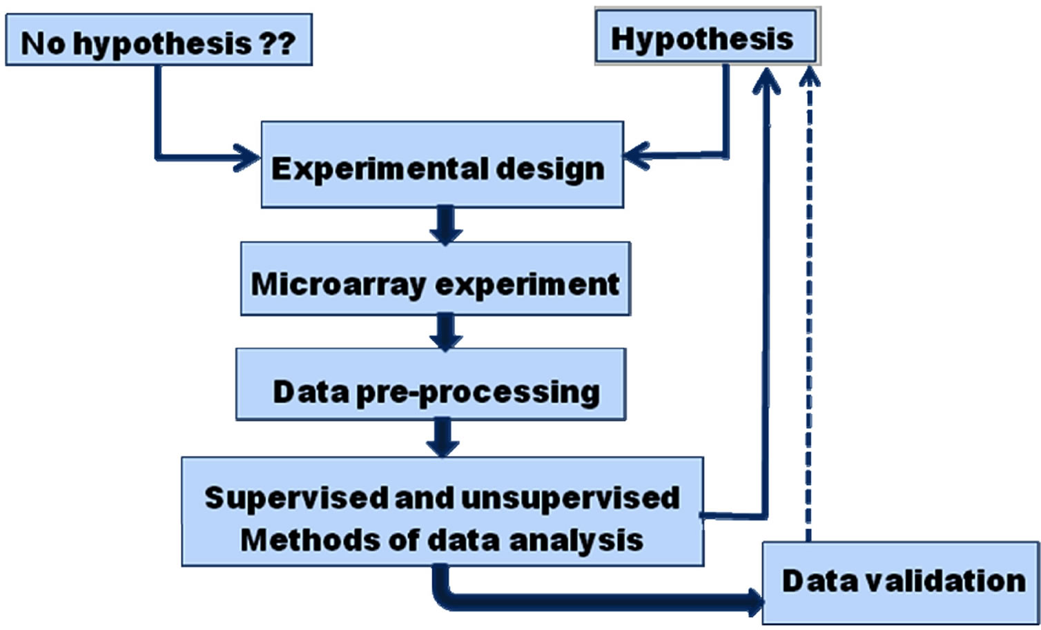
Figure 1. An overview of microarray experiment and data analysis. An experiment is designed according to the biological question it seeks to answer one may start with a hypothesis, i.e. expression of a particular set of genes may be used to identify a certain condition or without any hypothesis and may be exploratory in nature. Microarray experiment is carried out, the raw data obtained is cleaned, normalized and transformed, gene expression matrix is constructed and higher level analysis is performed to obtain biological insights.
regulated genes differently. Genes up-regulated by a factor of two have an expression ratio of 2, while those down-regulated by a factor of 2 have an expression ratio of ½ (0.5). As a result, down-regulated genes are compressed between 1 and 0 while up-regulated genes expand to cover the region between 1 and positive infinity, hence a logarithimic transformation is used, generally the logarithimic base being 2. The advantage of this transformation is that it treats upand down-regulated genes equivalently and produces a continuous spectrum of values for differentially expressed genes, i.e. log2(2) = 1 and log2(1/2) = −1. However, before transformation, one must first have an accurate method for comparing the measured expression levels between query and reference samples, and this is done by means of normalization. Normalization scales one or both of the measured expression levels of each gene to make them equivalent, and consequently the expression ratios derive from them [2]. Normalization approaches use either the complete set of arrayed genes or a control set, generally either a set of housekeeping genes or a set of exogenous spiked-in controls. The assumption made while using a control set is that genes are detected at constant levels in all the samples under comparison. However, this requires careful quantization of the initial RNA and fails to account for any variation-dependent expression level. Normalization may also be done by using regression algorithms, i.e. LOWESS regression or ranking ordering and distribution normalization [3]. These algorithms rely on the core assumption that the majority of genes on the microarray are not differentially expressed.
2. FINDING SIGNIFICANT GENES
After normalization and transformation the measurements of expression are combined into a log ratio for each sample, which describes numerically the extent to which the gene is differentially expressed, and whether it is up-regulated or down-regulated. To identify those that are consistently differentially expressed across all replicates under experimental condition one may choose a threshold, i.e. 2 fold differential expression and select those genes whose average differential expression is greater than that of threshold. But from a statistical perspective this is not a good approach because the average ratio does not take into account the sample size or variability within the sample (replicates or individuals). Hence a methodology known as hypothesis test is used to determine whether or not a gene is differentially expressed.
A hypothesis test builds a probabilistic model for the observed data based on what is known as null hypothesis which in this case is that there is no biological effect, i.e. The gene is not differentially expressed due to conditions under study, but results instead from differences between replicates or measurement errors. Using this model, it is possible to calculate the probability of observing a statistic, i.e. average fold change that is at least as extreme as the observed statistic in the data. This probability is known as p-value [4]. The smaller the p-value, less likely it is that the observed data have occurred by chance, and the more significant is the result. These hypothesis tests may be a t-test (paired or unpaired depending on sample), Wilcoxon sign-rank test, Wilcoxon rank-sum test or bootstrap test or in case of more complex experiments ANOVA or general linear models. Bootstrap analysis has the advantage that it does not require the data to be normally distributed and are thus robust to noise and experimental artifacts and it is also possible to use bootstrap for more complex analysis, i.e. ANOVA models and cluster analysis [5].
One may perform statistical tests on different individual genes and conclude whether genes are up or downregulated based on these tests. But in case of microarray experiment one has to apply these tests to many genes in parallel which has serious consequence known as multiplicity of p-values, for example if the p-value is 0.01, by definition of p-value, each gene would have 1 percent chance of having p-value of less than 0.01 and thus will be significant at the one percent level. If there are 10,000 genes on an array then there may be 100 significant genes at this level. This gives rise to an important question: how does one know that the gene that appears to be differentially expressed is truly differentially expressed? This is a deep problem in statistic and the p-values must be adjusted so as to have an acceptable false possible rate. Multiple test correction is made to estimate what fraction of the differentially expressed genes called to be significant are false positive. This is called the false discovery rate (FDR) [6], from FDR q-values are calculated which is something like a FDR-corrected version of the p-value [7]. The q-value for a particular test is the smallest FDR for which the test is rejected. Statistical softwares have sophisticated algorithms to perform these corrections. Application of such statistical filters is a key first step for further data mining [8] that is used for finding biological patterns in the data. Although statistical filters is not the same as biological significance, the genes that have the chance of being validated as differentially expressed are those which were found to be significant in statistical tests.
3. ANALYSIS OF DATA MATRIX
The goal of microarray data analysis is to find relationships and patterns in the data; to make further analysis convenient the expression data is represented as a matrix, where rows represent genes, columns represent experimental condition, and each value at each position in the matrix characterize the expression level of the particular gene under the particular experimental condition. Further additional information i.e. gene annotations, function descriptions or sample details may also be added to the matrix. After organizing the expression data into such matrices it can be used for higher level analysis. Current methodologies for higher level data analysis may be divided into two categories: Supervised approaches or analysis to determine genes that fit a determined pattern, they are used to find a “classifier” that separates data into classes; and Unsupervised approaches or analysis to characterize the components of a data set without a priori input or knowledge of the pattern and is used to find groups inherent to the data [9].
Most gene expression data analysis algorithms assume that the gene expression values are scalars; in these algorithms the replicates are either treated as separate experimental conditions or are replaced by one generalizing scalar, i.e. mean or median. Thus information about variance and reliability are lost. Another approach is to treat expression values as vectors where each gene can be considered as a point in m-dimensional space, where m is the number of samples. Similarly, each sample can be considered as a vector in n dimensional space where n is the number of genes. Thus all genes may be represented as points in multidimensional space and genes having similar expression values will be situated close to each other than genes having dissimilar expression values. This method provides an intuitive picture of similarity and mathematical formulae may be used to calculate “distance” between two expression vectors. There are varieties of methods for measuring distance, typically falling into three general classes: Euclidean, Non-Euclidean and semimetric [10].
When choosing a distance measure to use for further analysis, there is no one answers as to what is the best measure. Different measures have different strengths and weaknesses. Once the distance measure has been applied the expression matrix hence formed generally appears without any apparent pattern or order. Further analytical techniques may be applied to these matrices to re-order the rows or columns or both so that the pattern of expression becomes apparent. Among unsupervised techniques most common are—hierarchical clustering, k-means clustering, self-organizing maps.
3.1. Clustering
Clustering is a very useful technique for exploring expression patterns that exist in the data. Clustering results in grouping together of samples or genes having similar expression profiles. The data is divided into few groups thereby reducing the dimensionality in the data and making it more amiable for biological interpretation [11]. Hierarchical clustering is a commonly used unsupervised technique that builds clusters of genes with similar pattern of expression. This is done by iteratively grouping together genes that are highly correlated in terms of their expression measurements, then continuing the process on the groups themselves. Dendrograms are used to visualize the resultant hierarchical clustering (Figure 2). A dendrogram represents all genes as leaves of a large, branching tree. Each branch of the tree links two genes, two branches or one of each. Although construction of the tree is initiated by connecting genes that are most similar to each other, genes added later are connected to the branches that they most resemble. Although each branch links two elements, the overall shape of the tree may be asymmetrical. Branches connecting similar elements have shorter branch lengths while longer branches represent increasing dissimilarity (Figure 2). Hierarchical clustering is particularly advantageous in visualizing overall similarities in expression patterns observed in an experiment [12]. It is important to note the few disadvantages in their use: hierarchical clustering ignores negative association, even when underlying dissimilarity measure supports them. It does not result in clusters that are globally optimum, in that early incorrect choices in linking genes with a branch are not later reversible as the rest of the tree is constructed [2].
If there is prior knowledge regarding the number of clusters that should be represented in the data, K-means clustering is a good alternative to hierarchical methods [13,14]. In K-means, objects are partitioned into fixed number (K) of clusters such that the clusters internally are similar and externally are dissimilar. The process involved in K-means is conceptually simple but computationally intensive. Initially all objects are randomly assigned to one of the k clusters. An average expression
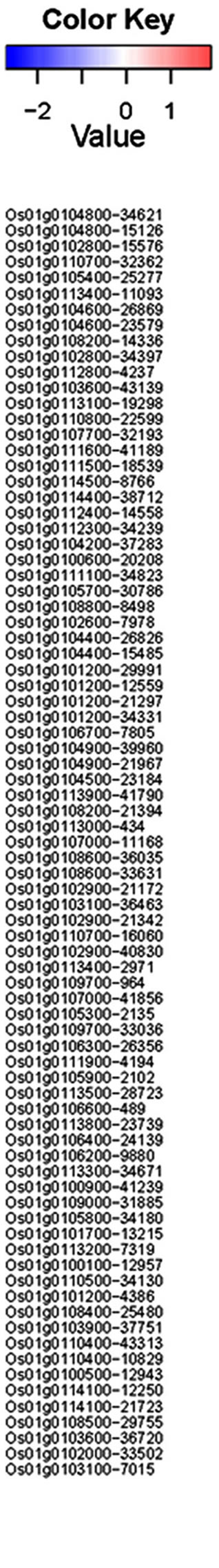

Figure 2. Hierarchical clustering. Dendrogram and heatmap depicting hierarchically clustered expression data of the first 100 loci on chromosome one of Oryzae sativa shoot after treatment with jasmonic acid at different time points (http://ricexpro.dna.affrc.go.jp).
vector is then calculated for each cluster, and this is used to compute the distances between clusters. Using an iterative method, objects are moved between clusters, intercluster distances are measured with each move. Objects are allowed to remain in the new cluster only if they are closer to it than to their previous cluster. After each move, the expression vectors for each cluster are recalculated. The shuffling proceeds until moving any more objects would make the clusters more variable (Figure 3) [15,16].
Self-organizing maps (SOM) are similar to hierarchical clustering, in that they also provide a survey of expression patterns within a data set, but the approach is quite different [17,18]. Genes are represented as points in multi dimensional space, and then genes are assigned to a series of partitions based on similarity of their expression vectors to reference vectors that are defined for each partition. It is the process of defining these reference vectors that distinguishes SOMs from k-means clustering. Before initiating the analysis, the user defines a geometrical configuration for the partitions, typically a twodimensional rectangular or hexagonal grid. A map is set with the centers of each cluster-to-be (known as centroids) arranged in the defined configuration. As the method iterates, the centroids move towards randomly chosen genes at a decreasing rate. The method continues until there is no further significant movement of these centroids. The advantages of SOM include easy twodimensional visualization of expression patterns [19] and reduced computational requirements compared with methods that require comprehensive pair wise comparisons. However, there are several disadvantages as well; the initial topology of a SOM is arbitrary and the movement of the centroids is random, so the final configuration of centroids might not be reproducible. Similar to dendrograms, negative associations are not easily found and even after the centroids reach the centers of each cluster, further techniques are needed to delineate the boundaries of each cluster.
Most of the clustering methods described above are heuristic in the sense that they do not try to optimize any scoring function describing the overall quality of the clustering. Model-based clustering assumes that the data have been generated by some, typically probabilistic

Figure 3. K-means clustering. A) Starting with three randomly placed centroids (green); B) Next, objects (red) are assigned to clusters nearest to them; C) Distance between objects and centroids is averaged out to move centroids to new location, resulting in new clusters; D) After each iteration the clusters are fed back into the same loop till the centroids converge.
(Bayesian), model and tries to find the clustering corresponding to the most probable model. They may still be heuristic in that they may not guarantee identification of the most probable clustering. Although model-based clustering has the potential to incorporate a priori knowledge about the domain in the analysis, it is not easy to apply it in a way that produces more meaningful biological results than purely heuristic methods. Fuzzy clustering is not deterministic, i.e. a given object either belongs or does not belong to a given cluster, but rather it assigns to each object the probability of belonging to the particular cluster [20]. Bayesian methods are often used for fuzzy clustering. The “goodness” of a cluster depends on how similar its objects are to each other and how dissimilar they are from next closest cluster. The most popular method for assessing the quality of clustering and for determining possible cut-off threshold is by shuffling the data, followed by clustering of shuffled data. However the ultimate proof of quality of clustering is the production of biologically meaningful results.
3.2. Principal Component Analysis
Principal component analysis (PCA) is another way of reducing dimensionality in the data. PCA is based on finding the direction in multidimensional vector space that has largest amplitude in the dispersion of data points i.e. greatest variability (Figure 4). This direction than serve as new co-ordinate axis and expression profiles are recalculated in this new transformed space. If only few
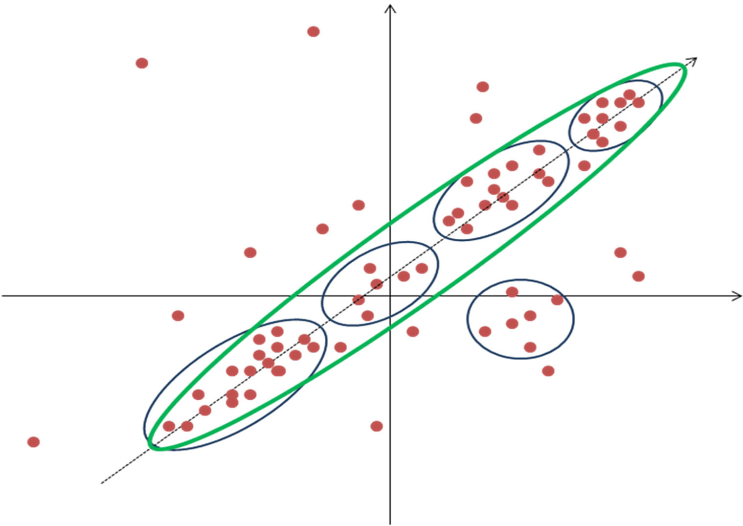
Figure 4. Principal component analysis. Data is divided into five clusters (blue) but only one principal component (green) is able to depict most of the dispersion. X and Y axis represent the gene expression values in two samples.
directions or principal components represent most of the variability then other directions are disregarded and hence dimensionality in data is greatly reduced. Principal components are a set of vectors in this space that decreasingly capture the variation seen in the points. The first principal component captures more variation than the second, and so on. Often in microarray datasets most variability can be accounted for by a small number of principal directions [21]. As each principal component exists in the same multidimensional space, they are linear combination of the genes or samples, the biological significance of these is not directly intuitive. Although principal components might best describe the variation seen in an expression data set, they do not describe how to best separate groups of genes or samples. Gene shaving is a clustering method that uses PCA [22,23]. It is an iterative heuristic method that works by alternating PCA and identifying the “best” clusters consisting of genes responsible for most of the variability in the data. The analysis starts by finding the first principal component; a mutually inclusive system of clusters is constructed starting with genes most similar to first principal component. The quality of clusters is estimated using “gapstatistics” [24] and the cluster with highest score is chosen. Next the gene space is transformed by removing component from each gene that is parallel to the first principle component. Gene shaving is different from other clustering methods discussed in that it does not produce exclusive clusters—a gene may belong to several clusters.
Multidimensional scaling (MDS) is a different approach to dimensionality reduction. Unlike PCA it does not start from the data, but rather uses the distance measures. It tries to locate the entities being compared in twoor three-dimensional space, as close as possible to the distances measured between the entities in the higher dimensional space [25,26].
3.3. Class Prediction
Supervised techniques use prior knowledge right from the beginning and try to find properties that support that knowledge. Generally here the focus is on finding genes that can be used for grouping samples into clinically or biologically relevant classes rather than on identifying gene functions. This is done by employing classification algorithms the simplest of them being linear regression and K-nearest neighbor methods. In linear regression “least square fit” is used to define a threshold line or linear space. Then a new point is classified into groups depending upon whether it lies below or above this thresh old. The K-nearest neighbor technique can be used in both supervised and unsupervised manner but the use of this technique in supervised fashion to find genes directly with patterns that best match a designated query pattern.
The query pattern may be an ideal gene pattern for a given condition, i.e. a group of genes that are highly expressed in one condition and expressed at a very low level in another condition. All the genes that have been measured can then be compared to this ideal gene pattern and ranked by their similarity [27,28]. Although this technique results in genes that might individually split two sets of microarrays, it does not necessarily find the smallest set of genes that most accurately splits the two sets. In other words, a combination of the expression levels of two genes might split two conditions perfectly, but these two genes might not necessarily be the top two genes that are most similar to the idealized pattern.
Support vector machines (SVM) address the problem of finding combination of genes that better split sets of biological samples [29]. Although it is easy to find individual genes that splits two sets with reasonable accuracy owing to the large number of genes (features) measured on microarrays, occasionally it is impossible to split sets perfectly using individual genes. The support vector machines based technique actually further expands the number of features available by combining genes using mathematical operations (called kernel functions). For example, in addition to using the expression levels of two individual genes A and B to separate two sets of biological samples, the combination features A×B, A/B, (A×B)2 and others can also be generated and used. It is possible even if genes A and B individually could not be used to separate the two sets of biological samples, together with the proper kernel function, they might successfully separate the two. In this technique each biological sample is considered as a point in multidimensional space, in which each dimension is a gene and the coordinates of each point is the expression level of that gene in the sample. Using SVM, this high-dimensional space gains even more dimensions representing the mathematical combinations of genes. The goal for SVM is to find a plane in this high-dimensional space that perfectly splits two or more sets of biological samples. Using this technique, the resulting plane has the largest possible margin from samples in the two conditions, therefore avoiding data over-fitting [30]. Although within this high-dimensional space, it is easier to separate samples from two or more conditions, but one problem is that the separating plane is defined as a function using all the dimensions available. For example, the most accurate plane to separate one disease from another might be (A×B)2 < 20, where A and B are expression levels of genes. SVM might be the most accurate way to separate two diseases but the biological significance of such functions is not always intuitive.
3.4. Biological Relevance
All The analytical techniques discussed so far end with a list of genes which would be meaningless without a biological context, this may be provided by using Gene Ontology (GO), an expert-curated database which assigns genes to various functional categories. GO is designed as a formal representation of biological knowledge, as it relates to genes and gene products [31]. It consists of three knowledge domains: molecular functions, biological processes and cellular component [32]. GO are based on evidence from literature, homology or other computational evidences including gene expression analysis, protein-protein interaction data, small nucleolar RNA prediction, domain prediction and similar techniques. GO is constantly expanded and revised in a collaborative manner to incorporate expanding knowledge. The analysis has to be carried beyond GO classification to delve deeper into the biological relevance of the subtle changes in gene expression. This may be done using relevance networks, pathway analysis or regulatory networks [32]. Relevance networks allow networks of features to be built, whether they represent genes, phenotypic or clinical measurements [33]. The technique works by first comparing measurements of all genes in a pair wise manner resulting in a pair wise calculation of mutual information. Thus each gene is completely connected to every other gene. Two genes are compared with each other by plotting all the samples on a scatter plot, using expression levels of the two genes as coordinates. A correlation coefficient is then calculated using any dissimilarity measure. Then a threshold mutual information is chosen based on permutation analysis and only those pairs of genes that have mutual information measure greater than threshold are kept. This results in clusters or more appropriately relevance networks that more strongly connected to each other. Relevance networks offer several advantages: they allow features of more than one data type to be represented together, features can have a variable number of associations, negative associations can be visualized as well as positive ones [34]. The only disadvantage is the degree of complexity seen at lower thresholds, at which many links are found associating many genes in a single network.
Pathway Analysis is used to map genes onto precompiled pathways to visualize whole chains of events indicated by microarray data [35]. The most relevant or tightly associated pathways may be highlighted using statistical tests, i.e. binomial, Chi-square tests, Fisher’s exact test [36] or hypergeometric distribution test [37]. The crucial shortcoming of pathway analysis is that, since it is derived from literature or precompiled pathways, it is unable to represent the underlying biological process completely. Regulatory networks are more appropriate in representing biological processes that involve more than one pathway by interconnecting pathways in a context specific manner [35,38]. In case of regulatory networks one must consider transcripts instead of genes and the associated genomic regulatory sequences (promoter and enhancers) and alternate transcripts. Several studies have been published [39-44] to approach molecular analysis of regulatory networks as stand alone or combined with GO and pathway analysis. However, application of regulatory to complex biological systems remains a complicated task requiring intensive preanalysis of sequences and comparative promoter analysis.
4. VISUALIZATION OF EXPRESSION DATA
One of the central features of microarray data is that there is a lot of it. No matter which distance measure is used one ends up with a high-dimensional data which is very difficult to comprehend. Thus to comprehend and visualize data it becomes necessary to reduce dimensionality of data through PCA or clustering. However, once the dimensionality has been reduced a number of visualization techniques may be used to find patterns in the data. The most popular techniques are heat maps (Figure 2), first introduced for gene expression data analysis by Michael Eisen [1]. A heat maps is simply a representative of the gene expression matrix using color coding, where the intensity of color represents the absolute values. Heat maps are typically used in association with clustering. Another popular way of depicting gene expression profiles and cluster of profiles is through the use of profile graphs. Profile graphs can be obtained by plotting expression values on the vertical axis, samples on the horizontal axis, and joining the points corresponding to the same genes in different samples. Another way in which covariance or gene expression datasets has been represented is gene expression terrain map. The covariance between datasets is calculated in large numbers of experiments using the expression levels of genes. The covariance is then represented in two dimensional space, such that closely related data are placed together and the altitude of the “gene mountain” represents the density of the gene at that site [45].
Correspondence analysis uses PCA in a chi-square distance matrix to allow one to assess which group of genes are most important for defining which experimental condition (sample) or vice-versa. It visualizes two or three principal axes of gene and sample space in the same diagram [46]. A rather different visualization approach is based on depicting the relationships among genes in the form of networks. Graph layout algorithms are used for visualizing gene expression networks. Visualization methods can also be used to combine gene expression data with other relevant data. Heat maps can be used in combination with gene ontology terms. Grid display is used to display gene expression in relation to position of the gene on the array [47]. Chromosome displays can be used to visualize the expression of genes in relation to their position along the chromosome [48].
5. RELATING HYPOTHESIS TO ANALYTICAL TECHNIQUE
Wide varieties of supervised and unsupervised methods are available for analysis, however, the existent challenge is in translating hypotheses into an appropriate bioinformatics technique. Supervised methods are of much use in domains of drug discovery and diagnostic testing, where definite answers are needed for specific questions. Unsupervised methods are less intuitive, because these start with less direct questions. These methods may be used to answer questions about the number and type of expression responses in a period of time after application of a compound. Hierarchical clustering and self-organizing maps survey all the genes and cluster them together on the basis of their expression patterns. Relevant networks may be used to search for the pairs of genes that are more likely to be co-expressed. True genetic regulatory networks might be found using methods such as constructing Bayesian networks. Moreover, a combination of both supervised and unsupervised methods may be used depending upon the answer that one seeks from the analysis, i.e. a hierarchical clustering may be used to obtain a dendrogram and then supervised learning may be used to find the best threshold to cut sub-trees or class vectors may be included into gene expression matrix as additional dimension and used for clustering. In all of the above cases, the analyses are not aimed at providing an ideal answer but are rather used as exploratory tools in the early discovery process.
The obvious truth with which one must agree after an experience with microarray technique is that the ratelimiting step in functional genomics is neither the actual experimental procedure nor the data analysis, but instead data interpretation for determining what the results actually mean. Detailed functional information might not yet be available for genes that have been found to be significant, even though these genes might be very well represented in microarray probe sets. The official name, predicted protein domains or gene-ontology classification might become available in a few days or might take decades. Oligonucleotide sequences that were thought to be unique at the time of designing the probe against a particular gene might not remain unique as more genomic data are collected. Operationally this means that one is never done analyzing a set of microarray data. The infrastructure has to be developed to reinvestigate constantly genes and gene information from microarray information performed in the past.
6. ACKNOWLEDGEMENTS
R.K.G is thankful to Council of Scientific and Industrial Research (F. No:09/015(0346)/2008-EMR-I) and Department of Biotechnology, Government of India for providing the financial assistance. Authors sincerely acknowledge Bose Institute for providing the infrastructure.