Runoff and Sediment Modeling Using SWAT in Gumera Catchment, Ethiopia ()
1. Introduction
Water is the foremost part of all living things, and a major force constantly shaping the surface of the earth. It is also a key factor in air conditioning of the earth for human existence and in influencing the progress of civilization, Ven Te Chow [1]. In Third World countries where the agricultural sector plays a key role in their economic growth, the management of water resource is an item of high priority in their developmental activities, K. Subramanian [2]. In Ethiopia where about 85% of the population is engaged primarily in agriculture and depends heavily on available water resources, the assessment and management of available water resources is a matter of prime importance. Surface water flow modelling is an important tool frequently used in studies in surface water system and watershed management and the modelling attempt to reproduce or simulate the operation of the real surface water system using mathematical models. The Gumera catchment is located in Amhara Region in the north-western Ethiopian Highlands wherein surface water utilization in and around this basin has been increased due to increasing urbanization and production of agricultural commodities. The Gumera catchment is one of the major catchments that significantly contributes to the livelihoods of millions of people around Lake Tana area and cover a total area of 1600 km2. This catchment is of critical national significance as it has great potentials for irrigation; high value crops and livestock production and others. It is therefore necessary to evaluate the existing trend and availability of surface water in time and space and its movement for proper planning in the near future.
The transformation of rainfall into stream flow is a complex process in Gumera catchment due to heterogeneities in topography, land cover and other catchment features. The present study is undertaken to model the stream flow and sediment yield behaviour in Gumera catchment using spatially distributed Soil and Water Assessment Tool (SWAT). The performance of the model in simulating runoff and sediment outflow is evaluated using SWAT Calibration and Uncertainty Program (SWAT-CUP).
2. Study Area
For the present study, Gumera catchment in Amhara regional state, northern highlands of Ethiopia (Figure 1) is chosen. Gumera River catchment is located within the latitude 11˚58'00"N & 11˚35'00"N and longitude 37˚50'00"E & 38˚11'00" and drains an area of 1600 km2 at its confluence with Lake Tana. Lake Tana is located in a wide depression of Ethiopian Plateau and is surrounded by high hills and mountains except where the outflow leaves the lake by a narrow valley in the south-east. The study area Gumera catchment is located in the eastern part of Lake Tana, the altitude varies within the range of 1784 to 3704 m above mean sea level. The topography of the watershed can be categorized in two main parts the upper most part of the watershed is mountainous and the lower part is relatively plain and gentle the general slope is from west to east.
The soils in most of the Tana basin are derived from the weathered basalt profiles, and are highly variable. In low lying areas particularly north and east of Lake Tana the soils have been developed on alluvial sediments [3]. The surface soil in the eastern part of the Gumera catchment is characterized with clay and clay loamy to clay, the central part is characterized as clay to silt clay and clay whereas the western part is silt clay and clay. Most of the Gumera catchment area is characterized by cropland with scarce woodlands while only few limited areas of highlands are forested (less than 1% of the catchment area). The major land cover types are dominantly cultivated lands (63.2%), Moderately Cultivated land (31%), Grassland (3.2%), Forest (0.36%), Urban and Built-Up (0.063%) and Water Body (0.059%).
In general there are three seasons in Ethiopia. The main rainy season is known locally as Kiremt (June-September), the dry season as Bega (October-January) and small rainy season as Belg (Februar-May). The Gumera catchment, in spite of being located near the equator, has a comparatively mild climate because of its high elevation (2794 m). The estimated mean annual precipitation ranges from 1200 to 1600 mm based on data from 1961 to 2000 (Gamachu, 1977; Conway, 2000; Kim, et al., 2008; Setegn, et al., 2009a) with more than 80% of annual rainfall falling during May to September. There is diurnal difference in temperature, but the temperature is comparatively uniform throughout the year with a mean annual temperature of 20.2˚C at Bahir Dar. The annual average daily maximum and minimum temperature (1994-2004) at Bahir Dar are 27.2˚C and 13.2˚C respectively.
The Lake Tana has more than 40 tributary rivers, but the major rivers feeding the lake are Gilgel Abay from the south, Ribb and Gumera from the east and Magetch River from the north, while there are no large rivers that flow from the western side of the lake. Among the above five major rivers Gumera river which is selected for this study has the annual runoff volume ranging from a minimum of 643 Mm3 (in 1987) to a maximum of 1691 Mm3 (in 1996) and with an average annual runoff volume of 1045 Mm3 (within the period 1981-2006).
2.1. ArcSWAT
ArcSWAT is a public domain graphical user interface program. It is designed to link the hydrologic model SWAT (Soil and Water Assessment Tool) and the GIS package ARC/INFO. The development of the interface was supported by Kansas Water Office and the University of Kansas General Research Fund.

Figure 1. Location of Gumera catchment and weather station distribution.
The SWAT model is limited in that it does not explicitly allow for the inclusion of spatial data as model inputs. Data must be processed into a form that the model can use. Processing these data, even with the use of a GIS, is tedious and time consuming due to the large number of model parameters required to execute SWAT.
The development of ARCSWAT aims at an effective use of spatial data to enhance hydrological modeling. The interface performs the following tasks: 1) to streamline GIS processes tailored toward SWAT modeling needs; 2) to automate data communication between Arc/Info and SWAT; and 3) to provide a user-friendly data entry and editing environment for SWAT [4].
2.2. SWAT Model
For the present study, SWAT (Soil and Water Assessment Tool) is used for modeling runoff and sediment outflow from study catchment. SWAT is a public domain hydrologic model, developed by USDA Agricultural Research Service. It is a semi-empirical and semi-physical model; it is a basin scale, continuous time, conceptual and long term simulation model that operates on daily and hourly time step. The SWAT is designed to simulate management impacts on water and sediment movement for un-gauged rural basins. It is computationally efficient and uses readily available input data such as weather, soil properties, topography, vegetation and land management practices occurring in the watershed. SWAT contains several hydrologic components (surface runoff, ET, recharge, stream flow, snow cover and snow melt, interception storage, infiltration, pond and reservoir water balance, and shallow and deep aquifers) that have been developed and validated at smaller scales (Williams, et al., 1984; Leonard, et al., 1987). Characteristics of this flow model include non-empirical recharge estimates, accounting of percolation, and applicability to basinwide management assessments with a multi-component basin water budget. A full description of SWAT can be found in the theoretical documentation by Neitsch, et al. [5], which is also available online. The model simulates a basin by dividing it into sub-watersheds that account for differences in soils and land use. The sub-basins are further divided into hydrologic response units (HRUs). These HRUs are the product of overlaying of slope, soils and land use. SWAT was evaluated by performing calibration and uncertainty analysis using SWAT-CUP.
2.3. SWAT-CUP
SWAT-CUP (SWAT Calibration and Uncertainty Procedures) is designed to integrate various calibration and uncertainty analysis programs for SWAT (Soil & Water Assessment Tool) using different interface. Currently the program can run SUFI2 (Abbaspour, et al., 2007), GLUE (Beven and Binley, 1992), and ParaSol (van Griensven and Meixner, 2006), PSO, and MCMC procedures. Currently the program links with Generalized Likelihood Uncertainty Estimation (GLUE), Parameter Solution (ParaSol) [6], Sequential Uncertainty Fitting (SUFI2), and Markov chain Monte Carlo (MCMC) procedures. For this study, various SWAT parameters related to discharge and sediment were estimated using the SUFI2 and ParaSol optimization technique. These optimization techniques uses the range of the parameters as constraints and 7 of the model evaluation coefficients as Objective Functions (OF) during calibration, they are 1) A multiplicative form of the square error (mult); 2) A summation form of the square error (sum); 3) Coefficient of determination (r2); 4) Nash-Sutcliffe (1970) coefficient (NS); 5) Chi-squared χ2 (Chi2); 6) Coefficient of determination R2 multiplied by the coefficient of the regression line (br2); and 7) sum of square of residual (SSQR). Only one objective function is used at a time during calibration time. In SUFI2 all of the OF are exist, there is also a possibility to improve the model evaluation coefficients by using different OF, but in ParaSol there is only one objective function that is SSQR. A full description of SWAT-CUP can be found in the [7].
2.4. Model Set up
The first step in setting up of SWAT model on any study area is the physiographic analysis based on catchment topography. The ArcSWAT automatically delineates a watershed into sub-watersheds based on Digital Elevation Model (DEM) to account for catchment heterogeneities. Pre-processed 90 m resolution DEM of the study area was supplied to the ArcSWAT for topographic analysis, delineation of sub-watershed and stream network generation. The whole catchment was divided into 24 subbasins as shown in Figure 2. Successful execution of terrain processing module of ArcSWAT interface resulted in generation of appropriate database for the sub-basin parameters and a detailed topographic report of the watershed.
Land use and soil map along with their respective look up tables prepared earlier were supplied to the model for reclassification according to SWAT coding convention.

Figure 2. Delineation of study area (Gumera River watershed).
Further entire watershed was classified into three slope categories using the interface. All three maps were then overlaid to create HRU’s with unique land cover/soil and slope class. Subdividing the areas into hydrologic response units enables the model to reflect the evapotranspiration and other hydrologic conditions for different land cover/crops and soil.
Location table of Weather Data, Daily Precipitation Data Files, Maximum and Minimum Temperatures, Wind Speed, Relative Humidity were loaded to link them up with the required files already created for the purpose. Due to lack of data on Solar Radiation, it was generated by model itself. After loading all the input data and generating the required database files, SWAT model was initially run on monthly basis using default parameter values.
2.5. Model Performance Evaluation
Results of the calibration and validation were evaluated based on the visual comparison and statistical criteria such as, Nash Sutcliffe Efficiency (NSE), Coefficient of Determination (R2), Relative Volume Error (% error), Root Mean Square Error (RMSE) and Mean Absolute Error (MAE), Sum of Square Residuals (SSQR), p-factor and r-factor. Some of the model performance coefficients this study frequently uses are described below.
2.5.1. Nash-Sutcliffe Coefficient [NS]
Nash-Sutcliffe coefficient measures the efficiency of the model by relating the goodness-of-fit of the model to the variance of the measured data, Nash-Sutcliffe efficiencies can range from −∞ to 1. An efficiency of 1 corresponds to a perfect match of modelled discharge to the observed data. An efficiency of 0 indicates that the model predictions are as accurate as the mean of the observed data, whereas an efficiency less than zero (−∞ < NS < 0) occurs when the observed mean is a better predictor than the model. Besides, due to frequent use of this coefficient, it is known that when values between 0.6 and 0.8 are generated, the model performs reasonably. A value between 0.8 and 0.9 tells that the model performs well and a value between 0.9 and 1 indicates that the model performs extremely well [8]. The formula for NashSutcliffe (NS) is:

where: ENS: Nash-Sutcliffe coefficient, qSi: simulated flow, qoi: observed flow and qo: average of observed flow.
2.5.2. Coefficient of Determination [R2]
The coefficient of determination, denoted r2, it provides a measure of how well observed outcomes are replicated by the model. The range of r2 lies between 0 and 1 which described how much of the observed desperation is explained by the prediction. A value of zero means no correlation at all; whereas one means that the desperation of the prediction is equal to that of the observation.
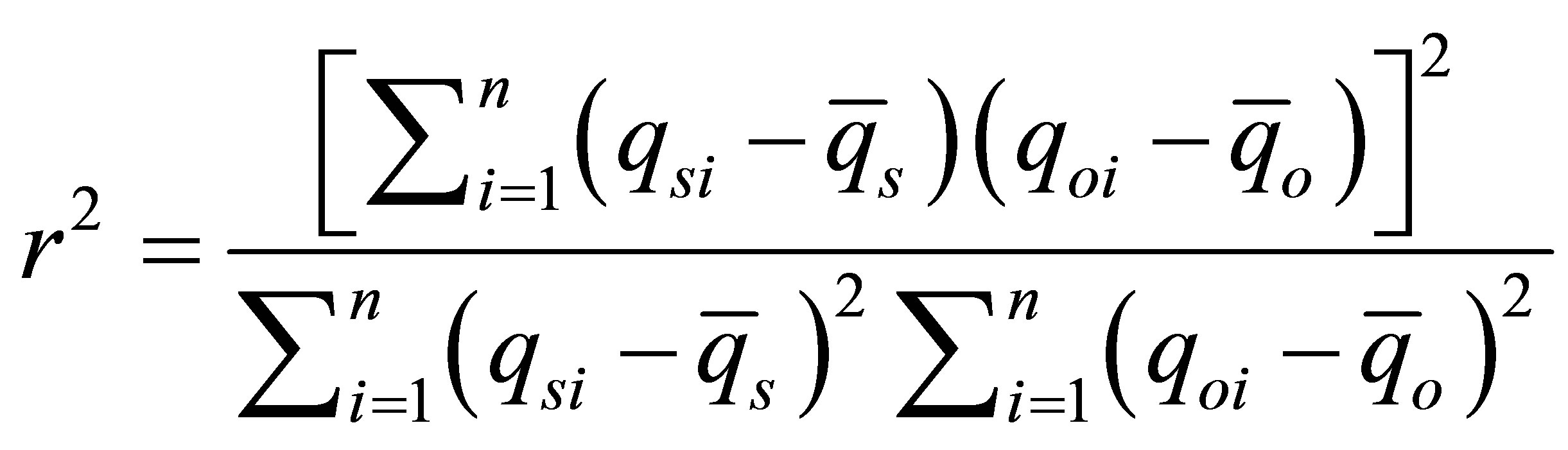
where: r2: coefficient of determination, qsi: simulated flow, qoi: observed flow and qo: average of observed flow.
2.5.3. Relative Volume Error [% Error]
The last performance measure, the RVE is used for quantifying the volume errors. This relative volume error can vary between positive infinitive and negative infinitive but when the value zero is generated it performs the best there is no difference between simulated and observed runoff occurs (Janssen and Heuberger, 1995). A relative volume error less than positive 0.05 or negative 0.05 indicates that a model performs is good while relative volume errors between +0.05% and +0.10% and −0.05% and −0.10% indicate a model with reasonable performance. This objective function should always be used in combination with another objective function that considers the overall shape agreement.
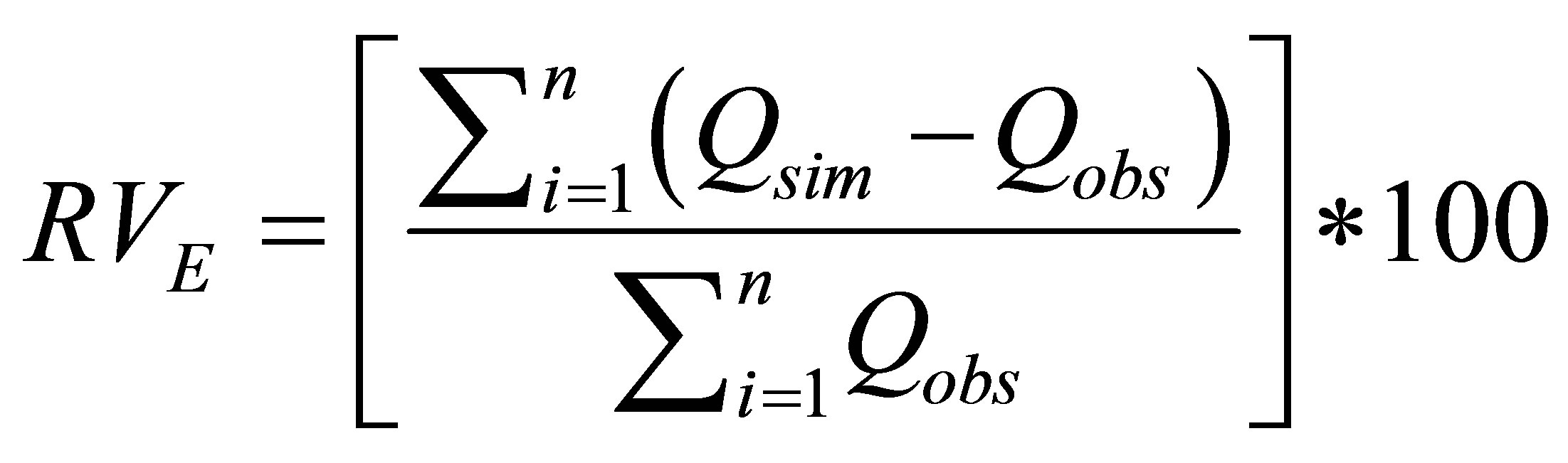
where: RVE (% error): relative volume error, QSim: simulated flow and Qobs: observed flow.
2.5.4. p-Factor and r-Factor
The degree to which all uncertainties are accounted for is quantified by a measure referred to as the p-factor, which is the percentage of measured data bracketed by the 95% prediction uncertainty (95PPU). Another measure quantifying the strength of a calibration/uncertainty analysis is the r-factor, which is the average thickness of the 95PPU band divided by the standard deviation of the measured data.
Theoretically, the value for p-factor ranges between 0 and 100%, while that of r-factor ranges between 0 and infinity. A p-factor of 1 and r-factor of zero is a simulation that exactly corresponds to measured data. The degree to which we are away from these numbers can be used to judge the strength of our calibration. A larger p-factor can be achieved at the expense of a larger rfactor. Hence, often a balance must be reached between the two. When acceptable values of r-factor and p-factor are reached, then the parameter uncertainties are the desired parameter ranges (SWAT-CUP 2012 user manual).
3. Results and Discussion
3.1. Model Calibration and Validation
The objective of calibration and validation was to maximizing the model efficiencies and finally using the parameter values obtained through those calibration techniques. This study uses ParaSol fully automated calibration technique and SUFI2 semi automated inverse modeling techniques. The calibration was performed using observed data from the year 1994 to 2002. The calibrated model was validated using independent data from 2003 - 2006, on daily and monthly time step at Gumera river gauge and discharge site.
Model Calibration and Validation Using ParaSol: The calibration was done using fully automated ParaSol interface which takes a wide parameter range as model constraints, the only objective function SSQR is used for this calibration and the number of simulations were more than 1000. The time series plot of measured daily and monthly flow simulated during calibration period for best simulations are shown on Figures 3 and 4 respectively and the summarized objective function results are also shown on Table 1. And to check the validity of the model, computed runoff have been compared with field observed flow data from 2003 to 2006.
The time series plot of measured daily and monthly flow simulated during validation period are shown on Figures 5 and 6 respectively and the summarized objective function results are also shown on Table 2. A scatter plot between monthly observed and simulated runoff is shown as Figure 7. As can be seen from Figure 7, most of the data points fall within 30% error bands.

Figure 3. Daily flow calibration plot (ParaSol).

Figure 4. Monthly flow calibration plot (ParaSol).

Table 1. Model performance evaluation coefficients for calibration of flow (ParaSol).

Table 2. Model performance evaluation coefficients for validation of flow (ParaSol).

Figure 5. Daily flow validation plot (ParaSol).

Figure 6. Monthly flow validation plot (ParaSol).

Figure 7. Monthly flow validation plot (ParaSol).
Model Calibrationand Validation Using SUFI2 Algorithm: Calibrated model predictive performance for Gumera River catchment is summarized in Table 3 and the time series plot of measured and simulated Monthly flow shows in Figure 8. This calibration was done using

Figure 8. Simulated and observed monthly flow superimposed with monthly rainfall (SUFI2).

Table 3. Model performance evaluation coefficients for calibration of monthly flow (SUFI2).
semi automated calibration technique by converging the parameter values in to very narrow range and use as model constraints, the default br2 was the objective function for this calibration and also the number of simulations is not more than 1000.
The time series plot of measured monthly flow simulated during validation period are shown on Figure 9 and the summarized model predictive performance values are on Table 4 a quit good match is found during daily and monthly time period. While when we go through each year by visual inspection and with model performance evolution coefficient, relative volume error (% error) shown in Table 9 especially for the years 1994, 1998 and 1999 the absolute value of % error is above 40% which is not good.
A scatter plot between monthly observed and simulated runoff is shown as Figure 10. As can be seen from the plot, most of the data points fall within 30% error bands.
3.2. Parameter Sensitivity Analysis
One-at-a-time sensitivity analysis: shows the sensitivity of a variable to the changes in a parameter if all other parameters are kept constant at some value. Parameter sensitivity (S) is expressed by a sensitivity index (SI) which is calculated as the ratio between the relative change of model output and the relative change of input parameter.

where, SI = Sensitivity Index, a dimensionless number; y represents model output function and x is the input parameter.
A one to one Sensitivity analysis is performing on this study with changing the value of calibrated 13 parameters (CN2, ESCO, SOL_K, SOL_AWC, SOL_Z, CH_N2, ALPHA_BF, ALPHA_BF, GW_DELAY, GWQMN, GW_REVAP, REVAPMN, RCHRG_DP and SURLAG) One-at-a-time. Table 5 shows the values of sensitivity index (SI) for different input parameters. For most of the parameters Δx% was taken as 25% except for those parameters where 25% change causes a value which exceeds the parameter valid range. All the input parameters tested for Gumera watershed in terms of their impact on three model outputs of total water yield (TWYLD), surface runoff (SURQ) and subsurface flow (LATQ + GWQ) or base flow, six parameters CN2, ESCO, SOL_AWC, GWQMN, SOL_K and GW_REVAP found to be sensitive parameters out of 13 tested input parameter, as per the classification proposed by Lnehart, et al., 2002.
The absolute value of SI for the parameters like CN2 and ESCO towards water yield greater than one shows very high sensitive nature towards the total water yields (TWYLD) and parameter like SOL_AWC is highly sensitive towards model water yield having absolute SI value between 0.20 < SI < 1.00, Whereas parameters like GWQMN, SOL_K and GW_REVAP are medium sensitive towards model water yield having absolute SI ranges between (0.05 and 0.13). SOL_AWC, GWQMN, SOL_K

Figure 9. Monthly flow validation plot (SUFI2).

Figure 10. Monthly flow validation plot (SUFI2).

Tabel 4 . Model performance evaluation coefficients for validation of monthly flow (SUFI2).
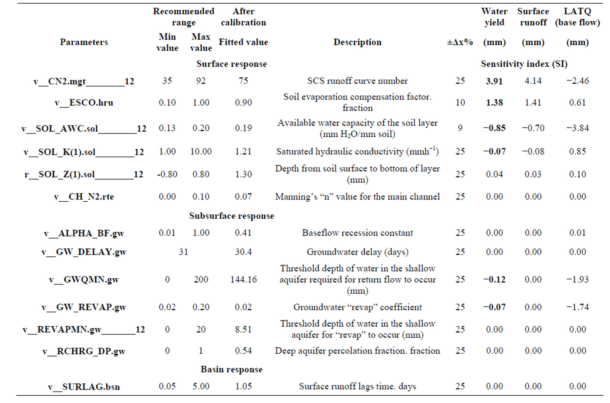
Table 5. One-at-a-time sensitivity analysis.

Table 6. Increasing parameter value TWYLD decreases, when SI value negative.
and GW_REVAP have negative SI values −0.85, −0.12, −0.07, and −0.07 respectively, their negative sign shows that on increasing parameter value TWYLD decreases, Table 6 shows an example of SOL_AWC parameter.
3.3. Estimation of Daily Sediment Load Using LOADEST
Suspended-sediment data from one selected surface-water monitoring stations in the Gumera River Basin (Gumera near Bahr-Dar station) were used in the computation of daily suspended-sediment for 1992 through 2006, by using regression techniques built-in the Load Estimator (LOADEST) software by characterizing the suspended-sediment and stream flow data collected at the selected monitoring stations. The results produced with LOADEST are shown in Figure 11.


Figure 11. Daily sediment load by (LOADEST) superimposed with daily flow at Gumera station.
3.4. Model Calibration and Validation with Monthly Sediment Load
The Sediment calibration was done after fixing 13 calibrated runoff parameters and then adding four additional parameters by using SUFI2 calibration technique in monthly time scale. The time series plot of model calibration and validation for monthly sediment load are shown in Figures 12 and 13 respectively and model performance evaluation is shown on Tables 7 and 8 respectively.
In general the R2 and Nash Sutcliff coefficients (NSE) values are above 50%, for prediction sediment yield these performance evaluation coefficients values are in acceptable range. While when we see in individual year sediment load comparison in Table 9 by using relative volume error method, especially for the years 1996, 1998, 1999 and 2005 the absolute value of % error is above 40%.
4. Summary and Conclusions
In the present study, SWAT 2005, a process based partially distributed hydrological model having an interface with ArcGIS software was used for modelling runoff and sediment load from Gumera River watershed in Ethiopia. After preparing all required thematic maps and database as per the format of ArcSWAT model, model was setup and calibrated for the daily and monthly total water yield and sediment load using the observed data of 1994 to 2002. The model validation was carried out for a data set of four years from 2003 to 2006. The performance of the model for calibration and validation was evaluated using graphical and statistical methods.
The coefficient of determination R2 and NS coefficient for the daily runoff using [ParaSol] was 0.72 and

Table 7. Model performance evaluation coefficients for calibration of monthly Sediment yield (SUFI2).

Table 8. Model performance evaluation coefficients for validation of monthly Sediment yield (SUFI2).
0.71 respectively within nine years calibration period and 0.79 and 0.78 respectively for four year validation period, the value of the coefficients using SUFI2 for monthly flow is R2 = 0.83 and NS = 0.79 for the calibration period R2 = 0.93 and NS = 0.93 for the validation period. For sediment yield using [SUFI2] algorithm during calibration was computed as R2 = 0.61 and NS = 0.60, for validation it was R2 = 0.84 and NS = 0.83. The model performance evaluation coefficients shown in this study can be considered reasonably satisfactory and the SWAT model is capable of predicting runoff and sediment yields from Gumera catchment with limited data availability. Finally SWAT Model is available and user-friendly in handily input data, SWAT was evaluated by performing calibration and uncertainty analysis, while it needs reliable input data and sufficient time for obtaining improved model parameters, when we see the SUFI2 calibration it is more flexible than PraSol any time can change the objective function and can be adjusted the

Figure 12. Monthly sediment calibration plot (SUFI2).

Figure 13. Monthly sediment validation plot (SUFI2).

Table 9. Relative volume error (% error) values for calibrated and validated yearly flow and sediment load.
parameter range during calibration and SUFI2 consider all model uncertainty.