On Existence of Periodic Solutions of Certain Second Order Nonlinear Ordinary Differential Equations via Phase Portrait Analysis

Olaniyi S. Maliki¹, Ologun Sesan²

¹Department of Mathematics, Michael Okpara University of Agriculture, Umudike, Nigeria.
²Department of Mathematics, University of Uyo, Uyo, Nigeria.

DOI: 10.4236/am.2018.911080                

Abstract

The global phase portrait describes the qualitative behaviour of the solution set of a nonlinear ordinary differential equation, for all time. In general, this is as close as we can come to solving nonlinear systems. In this research work we study the dynamics of a bead sliding on a wire with a given specified shape. A long wire is bent into the shape of a curve with equation z = f (x) in a fixed vertical plane. We consider two cases, namely without friction and with friction, specifically for the cubic shape f (x) = x³−x . We derive the corresponding differential equation of motion representing the dynamics of the bead. We then study the resulting second order nonlinear ordinary differential equations, by performing simulations using MathCAD 14. Our main interest is to investigate the existence of periodic solutions for this dynamics in the neighbourhood of the critical points. Our results show clearly that periodic solutions do indeed exist for the frictionless case, as the phase portraits exhibit isolated limit cycles in the phase plane. For the case with friction, the phase portrait depicts a spiral sink, spiraling into the critical point.

Keywords

ODE, Stability, Periodic Solutions, Limit Cycles, MathCAD Solution

1. Introduction

Nonlinear dynamical systems exhibiting oscillating limit cycles are found in a large variety of fields including biology, chemistry, mechanics and electronics, [1] [2] . The historical development of the study of periodic solutions of ordinary differential equations began in a series of articles published in the 19^th century. It was Henri Poincare that initiated the qualitative theory of differential equations. This qualitative approach was intended both to guide and bring to light the limits of numerical methods, such as the series solutions, which was quite popular at the time. Most of the qualitative investigations were generally of a local character. Thus, the behaviour of solution is studied in a sufficiently small neighborhood of a given solution, for example in a neighborhood of stationary point or of a periodic solution.

A bead sliding on a wire is a classic problem in theoretical dynamics [3] . Our interest in this problem is from the point of view of studying the resulting nonlinear differential equations. We seek in particular periodic solutions as well as stability properties, using phase portrait analysis. Furthermore, the shape of our wire is specified by a general curve $z=f\left(x\right)$ , and hence we can study different configurations of the given problem.

The temporal evolution of a dynamical system is usually described by points in space and time. The line joining all these points is called the trajectory. A trajectory that comes back upon itself to form a closed loop in phase space is called an orbit [4] . An orbit for a system usually indicates that the dynamical system under consideration is conservative. We also note that each plotted point along any trajectory has evolved directly from the preceding point. As we plot each successive point in phase space, the plotted points migrate around. Orbits and trajectories therefore reflect the movement or evolution of the dynamical system.

The phase space plot is a world that shows the trajectory and its development. Depending on various factors, different trajectories can evolve for the same system. The phase space plot and such a family of trajectories together are a phase space portrait, phase portrait, or phase diagram.

2. Limit Cycles and Other Closed Paths

The world we live in can be described more accurately by systems of nonlinear differential equations. Furthermore, in nonlinear systems there is particular interest in the existence of periodic solutions, as well as their amplitudes, periods, and phases. If the system is autonomous, and $x\left(t\right)$ in any solution, so is $x\left(t+\tau \right)$ for any value of $\tau$ , which means that phase is not significant since the solutions map on to the same phase paths. In the phase plane, periodic solutions appear as closed paths [5] . Conservative systems and Hamiltonian systems are essentially energy systems, and often contain nests of closed paths forming centres, which we might expect since they are generally non-dissipative; meaning that friction is absent.

A limit cycle is an isolated periodic solution of an autonomous system [6] , represented in the phase plane by an isolated closed path. The neighbouring paths are, by definition, not closed, but spiral into or away from the limit cycle. Furthermore, for a stable limit cycle, the device represented by the system, which might be, for example, an electronic circuit, will spontaneously drift into the corresponding periodic oscillation from a wide range of initial states. The existence of limit cycles is therefore a feature of great practical importance.

3. Statement of the Problem

We derive the differential equation of motion of a bead of mass m, sliding on a wire of given shape $z=f\left(x\right)=x^3-x$ in the vertical plane. We consider two cases, namely without friction and with friction. For both cases we perform simulation of the derived differential equations. Our interest is to study the resulting nonlinear ordinary differential equations, and investigate the existence of periodic solutions for this dynamics in the neighbourhood of the critical points. This will be depicted by their corresponding phase portraits.

4. Gradient and Hamiltonian Systems

Let E be an open subset of ${ℝ}^{2n}$ and let $H\in C^2\left(E\right)$ where $H=H\left(x,y\right)$ with $\forall x,y\in {ℝ}^n$ . A system of the form

$\stackrel{\dot{}}{x}=\frac{\partial H}{\partial y}\text{,}\stackrel{\dot{}}{y}=-\frac{\partial H}{\partial x}$ (1)

where

$\frac{\partial H}{\partial x}={\nabla }_{x}H\text{and}\frac{\partial H}{\partial y}={\nabla }_{y}H$

is called a Hamiltonian system with n degrees of freedom on E. For example, the Hamiltonian function

$H\left(x,y\right)=\frac{1}{2}\left(x_1^2+x_2^2+y_1^2+y_2^2\right)$ (2)

is the energy function for the spherical pendulum

${\stackrel{\dot{}}{x}}_1=y_1,{\stackrel{\dot{}}{x}}_2=y_2$

${\stackrel{\dot{}}{y}}_1=-x_1,{\stackrel{\dot{}}{y}}_2=-x_2$

This system is equivalent to the pair of uncoupled harmonic oscillators;

${\ddot{x}}_1+x_1=0,{\ddot{x}}_2+x_2=0$

All Hamiltonian systems are conservative in the sense that the Hamiltonian function or the total energy $H\left(x,y\right)$ remains constant along trajectories of the system.

5. Theorem (Conservation of Energy)

The total energy $H\left(x,y\right)$ of the Hamiltonian system (1) remains constant along its trajectories.

Proof

The total derivative of the Hamiltonian function $H\left(x,y\right)$ along a trajectory $x\left(t\right),y\left(t\right)$ of (1)

$\frac{\text{d}H}{\text{d}t}=\frac{\partial H}{\partial x}\cdot \stackrel{\dot{}}{x}+\frac{\partial H}{\partial y}\cdot \stackrel{\dot{}}{y}=\frac{\partial H}{\partial x}\cdot \frac{\partial H}{\partial y}-\frac{\partial H}{\partial y}\cdot \frac{\partial H}{\partial x}=0$

Thus, $H\left(x,y\right)$ is constant along any solution curve of (1) and the trajectories of (1) lie on the surfaces $H\left(x,y\right)$ = constant.

6. Remark

We now establish some very specific results about the nature of the critical points of Hamiltonian systems with one degree of freedom. Note that the equilibrium points or critical points of the system (1) correspond to the critical points of the Hamiltonian function $H\left(x,y\right)$ where $\partial H/\partial x=\partial H/\partial y=0$ . We may, without loss of generality, assume that the critical point in question has been translated to the origin.

7. Lemma

If the origin is a focus of the Hamiltonian system

$\stackrel{\dot{}}{x}=H_y\left(x,y\right),\stackrel{\dot{}}{y}=-H_x\left(x,y\right)$ (3)

then, the origin is not a strict local maximum or minimum of the Hamiltonian function $H\left(x,y\right)$ .

8. Definition

A critical point of the system $\stackrel{\dot{}}{x}=f\left(x\right)$ at which $Df\left(x_0\right)$ (Jacobian) has no zero eigenvalues is called a non-degenerate critical point of the system, otherwise, it is called a degenerate critical point of the system.

9. Remark

We note that any non-degenerate critical point of a planar system is either a hyperbolic critical point of the system or a center of the linearized system.

10. Hamiltonian with One Degree of Freedom

One particular type of Hamiltonian system with one degree of freedom is the Newtonian system with one degree of freedom,

$\stackrel{\dot{}}{x}=f\left(x\right)$ (4)

where $f\in C^1\left(a,b\right)$ . This differential equation can be written as a system in ${ℝ}^2$ :

${\stackrel{\dot{}}{x}}_1=x_2,{\stackrel{\dot{}}{x}}_2=f\left(x_1\right)$ (5)

The total energy for this system $H\left(x_1,x_2\right)=T\left(x_2\right)+V\left(x_1\right)$ where $T\left(x_2\right)=x_2^2/2$ is the kinetic energy and

$V\left(x_1\right)=-{\displaystyle {\int }_{x_0}^{x_1}f\left(s\right)\text{d}s}$

is the potential energy. With this definition of $H\left(x_1,x_2\right)$ we see that the Newtonian system (4) can be written as a Hamiltonian system. It is not difficult to establish the following facts for the Newtonian system (4).

11. Theorem

The critical points of the Newtonian system (4) all lie on the x-axis. The point $\left(x_0,0\right)$ is a critical point of the Newtonian system (4) if and only if it is a critical point of the function $V\left(x_1\right)$ , i.e., a zero of the function $f\left(x\right)$ . If $\left(x_0,0\right)$ is a strict local maximum of the analytic function $V\left(x_1\right)$ , it is a saddle for (4). If $\left(x_0,0\right)$ is a strict local minimum of the analytic function $V\left(x_1\right)$ , it is a center for (4). If $\left(x_0,0\right)$ is a horizontal inflection point of the function $V\left(x_1\right)$ , it is a cusp for the system (4). Finally, the phase portrait of (4) is symmetric with respect to the x-axis.

12. Existence of Periodic Solutions

The existence of periodic solutions or otherwise of a system of ODE is settled in the following theorem.

13. Theorem

Consider the 2-dimensional autonomous system $\stackrel{\dot{}}{u}=f\left(u\right)$ where $f\left(u\right)\in C^1\left({ℝ}^2\right)$ . Let $\Omega \in {ℝ}^2$ be simply connected, such that $\forall u\in \Omega$ , we have $\text{div}f\left(u\right)=0$ . We now show that the ODE system has no periodic solutions in Ω.

Proof

Towards a contradiction, assume ODE system has a periodic solution in Ω. Let ∂Ω be a boundary on Ω.

$\stackrel{\dot{}}{u}=f\left(u\right)\Rightarrow \{\begin{array}{l}{\stackrel{\dot{}}{u}}_1=f_1\left(u_1,u_2\right)\\ {\stackrel{\dot{}}{u}}_2=f_2\left(u_1,u_2\right)\end{array}$

$n\equiv \left(n_1,n_2\right)=\left({\stackrel{\dot{}}{u}}_2,-{\stackrel{\dot{}}{u}}_1\right)$ is the normal to ∂Ω. Recall then Divergence Theorem:

${\displaystyle \underset{\partial \Omega }{\oint }f\cdot n\text{d}s}={\displaystyle \underset{\Omega }{\iint }divf\text{d}A}$

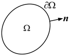
Let u be a periodic solution with period T, i.e. $u\left(t+T\right)=u\left(t\right)$ . Then, a path traversed by a solution starting from $t=a$ to $t=a+T$ is ∂Ω. Then, ∂Ω is a closed curve.

${\displaystyle \underset{\partial \Omega }{\oint }f\cdot n\text{d}s}={\displaystyle \underset{\partial \Omega }{\int }\left(f_1{n}_1+f_2{n}_2\right)\text{d}s}={\displaystyle \underset{a}{\overset{a+T}{\int }}\left({\stackrel{\dot{}}{u}}_1{\stackrel{\dot{}}{u}}_2-{\stackrel{\dot{}}{u}}_2{\stackrel{\dot{}}{u}}_1\right)\text{d}t}=0$

$\Rightarrow {\displaystyle \underset{\Omega }{\iint }divf}\text{d}A=0$

However, by hypothesis, $divf\left(u\right)\ne 0$ and $f\in C^1$ . Therefore, $divf\in C^0$ , and either $divf>0$ or $divf<0$ on Ω. Thus, ${\displaystyle {\iint }_{\Omega }divf\text{d}A}>0$ or ${\displaystyle {\iint }_{\Omega }divf\text{d}A}<0$ , a contradiction.

14. Remark

We can now state formally a theorem on the Bendixson criterion for the existence or otherwise of periodic solutions [7] .

15. Theorem (Bendixson Criterion)

Suppose that the domain $D\subset {ℝ}^2$ is simply connected; $\left(f,g\right)$ is continuously differentiable in D.

Then the equations

$\stackrel{\dot{}}{x}=f\left(x,y\right),\stackrel{\dot{}}{y}=g\left(x,y\right)$

can only have periodic solutions if $\nabla \cdot \left(f,g\right)$ changes sign in D or if $\nabla \cdot \left(f,g\right)=0$ in D.

16. Example

We know that the damped linear oscillator contains no periodic solutions.

Consider now a nonlinear oscillator with nonlinear damping represented by the equation

$\ddot{x}+p\left(x\right)\stackrel{\dot{}}{x}+q\left(x\right)=0$

We assume that $p\left(x\right)$ and $q\left(x\right)$ are smooth and that $p\left(x\right)>0$ , $x\in ℝ$ (damping). The vectorized system is

${\stackrel{\dot{}}{x}}_1=x_2,{\stackrel{\dot{}}{x}}_2=-q\left(x_1\right)-p\left(x_1\right)x_2$

$divf\left(x_1,x_2\right)=\frac{\partial f_1}{\partial x_1}+\frac{\partial f_2}{\partial x_2}=\frac{\partial }{\partial x_1}\left(x_2\right)+\frac{\partial }{\partial x_2}\left(-q\left(x_1\right)-p\left(x_1\right)x_2\right)=-p(x1)$

Thus the divergence of the vector function is $-p\left(x\right)$ which is negative definite. It follows from Bendixson’s criterion that the equation has no periodic solutions.

17. Derivation of the Main Models

Case 1: Smooth wire (no friction)

The bead and wire are shown in Figure 1. The components of the velocity of the bead are given by $\left(\stackrel{\dot{}}{x},\stackrel{\dot{}}{z}=f^{\prime }\left(x\right)\stackrel{\dot{}}{x}\right)$ . The kinetic and potential energies are

Figure 1. Bead sliding on frictionless wire.

$T=\frac{1}{2}m\left({\stackrel{\dot{}}{x}}^2+{\stackrel{\dot{}}{z}}^2\right)=\frac{1}{2}m\left(1+f^{\prime }{\left(x\right)}^2\right)y^2$ , $V=mgy=mgf(x)$

where $y=\stackrel{\dot{}}{x}$ .

Hence the Hamiltonian (total energy) H of the bead is

$H=T+V=\frac{1}{2}m\left(1+f^{\prime }{\left(x\right)}^2\right)y^2+mgf\left(x\right)$ (6)

The equation of motion of the bead can now be derived from the conservation principle of the total energy, i.e. $\stackrel{\dot{}}{H}=\text{d}H/\text{d}t=0$ . Hence assuming $f^{\prime }\left(x\right)$ and $f^{″}\left(x\right)$ are continuous,

$\stackrel{\dot{}}{H}=\frac{1}{2}m\frac{\text{d}}{\text{d}t}\left\{\left(1+f^{\prime }{\left(x\right)}^2\right)y^2\right\}+mg\frac{\text{d}}{\text{d}t}f\left(x\right)=0$

$\Rightarrow \left(1+f^{\prime }{\left(x\right)}^2\right)\stackrel{\dot{}}{y}+f^{\prime }\left(x\right)f^{″}\left(x\right)y^2+g{f}^{\prime }\left(x\right)=0$

Hence the differential equation of motion of the bead is;

$\left(1+f^{\prime }{\left(x\right)}^2\right)\ddot{x}+f^{\prime }\left(x\right)f^{″}\left(x\right){\stackrel{\dot{}}{x}}^2+g{f}^{\prime }\left(x\right)=0$ (7)

Case 2: Non-smooth wire (friction)

Let R be the normal reaction of the bead on the wire and let F be the frictional force opposing the motion as shown in Figure 2. The horizontal and vertical equations of motion are

$m\ddot{x}=-R\sin \theta -F\cos \theta$ (8)

$m\ddot{z}=R\cos \theta -mg-F\sin \theta$ (9)

where θ is the inclination of the tangent of the curve at the bead. Since $z=f\left(x\right)$ , then $\stackrel{\dot{}}{z}=f^{\prime }\left(x\right)\stackrel{\dot{}}{x}$ and $\ddot{z}=f^{″}\left(x\right){\stackrel{\dot{}}{x}}^2+f^{\prime }\left(x\right)\ddot{x}$ . Eliminating R between (12) and (13) gives;

$m\left(f^{″}\left(x\right){\stackrel{\dot{}}{x}}^2+f^{\prime }\left(x\right)\ddot{x}\right)+m\ddot{x}\cos \theta =-\left(mg+k\stackrel{\dot{}}{x}{f}^{\prime }\left(x\right)\right)\sin \theta -F$

where $\sin \theta =f^{\prime }\left(x\right){\left(1+f^{\prime }{\left(x\right)}^2\right)}^{-\frac{1}{2}}$ and $\cos \theta ={\left(1+f^{\prime }{\left(x\right)}^2\right)}^{-\frac{1}{2}}$ .

The frictional force F is proportional to the velocity and opposes the motion, hence

$F=-k\left(\stackrel{\dot{}}{x}\cos \theta +\stackrel{\dot{}}{z}\sin \theta \right)=-k\stackrel{\dot{}}{x}\sqrt{1+f^{\prime }{\left(x\right)}^2}$ (10)

Figure 2. Bead sliding on rough wire.

Therefore, the equation of motion is

$m\left(1+f^{\prime }{\left(x\right)}^2\right)\ddot{x}+m{f}^{″}\left(x\right)f^{\prime }\left(x\right){\stackrel{\dot{}}{x}}^2+k\stackrel{\dot{}}{x}\left(1+f^{\prime }{\left(x\right)}^2\right)+mg{f}^{\prime }\left(x\right)=0$ (11)

We observe that we obtain Equation (7) when we set $k=0$ for the frictionless wire.

18. Results: Bead Sliding on a Cubic Shaped Wire

Consider the case without friction, and the initial shape of the wire is a simple cubic given by $f\left(x\right)=x^3-x$ . The equation of motion of the bead is written;

$m\left(1+f^{\prime }{\left(x\right)}^2\right)\ddot{x}+m{f}^{″}\left(x\right)f^{\prime }\left(x\right){\stackrel{\dot{}}{x}}^2+k\stackrel{\dot{}}{x}\left(1+f^{\prime }{\left(x\right)}^2\right)+mg{f}^{\prime }\left(x\right)=0$

with $f^{\prime }\left(x\right)=3x^2-1$ , and $f^{″}\left(x\right)=6x$ . We examine two cases, viz;

1) For the frictionless case $k=0$ , and setting $m=1$ , $g=10$ we get

$\left(9x^4+6x^2+2\right)\ddot{x}+\left(18x^3-6x\right){\stackrel{\dot{}}{x}}^2+10\left(3x^2-1\right)=0$ (12)

2) For the case with friction $k=1$ , and the equation of motion reads;

$\left(9x^4+6x^2+2\right)\ddot{x}+\left(18x^3-6x\right){\stackrel{\dot{}}{x}}^2+\left(9x^4+6x^2+2\right)\stackrel{\dot{}}{x}+10\left(3x^2-1\right)=0$ (13)

Vectorizing Equations (12) and (13), we obtain respectively;

$\{\begin{array}{l}{\stackrel{\dot{}}{x}}_1=x_2\\ {\stackrel{\dot{}}{x}}_2=-\frac{\left(18x_1^3-6x_1\right)x_2^2+10\left(3x_1^2-1\right)}{9x_1^4+6x_1^2+2}\end{array}$ (14)

and

$\{\begin{array}{l}{\stackrel{\dot{}}{x}}_1=x_2\\ {\stackrel{\dot{}}{x}}_2=-\frac{\left(18x_1^3-6x_1\right)x_2^2+x_2\left(9x_1^4+6x_1^2+2\right)+10\left(3x_1^2-1\right)}{9x_1^4+6x_1^2+2}\end{array}$ (15)

19. Simulation of the Models Using MathCAD [8]

Case 1 (without friction)

We consider the vectorized systems of differential Equations (14)

Define a function that determines a vector of derivative values at any solution point (t, Y):

$D\left(t,Y\right):=\left[\begin{array}{c}{Y}_1\\ -\frac{{\left[18\cdot {\left(Y_0\right)}^3-6\cdot \left(Y_0\right)\right]}^2+\left[3\cdot {\left(Y_0\right)}^2-1\right]\cdot 10}{\left[9\cdot {\left(Y_0\right)}^4-6\cdot {\left(Y_0\right)}^2+2\right]}\end{array}\right]$

Additional arguments for the ODE solver are:

$t0:=0$ Initial value of independent variable;

$t1:=10$ End value of independent variable;

$Y\text{0}:=\left(\begin{array}{c}0.001\\ 0.001\end{array}\right)$ Vector of initial function values;

$N:=2\times {10}^3$ Number of solution values on [t0, t1].

Solution matrix:

$S1:=\text{Rkadapt}\left(Y0,t0,t1,N,D\right)$

$t:=S{1}^{\langle 0\rangle }$ Independent variable values;

$x1:=S{1}^{\langle 1\rangle }$ First solution function values;

$x2:=S{1}^{\langle 2\rangle }$ Second solution function values.

We have the following graphical profiles (Table 1).

Case 2 (with friction)

We now consider the vectorized nonlinear systems of differential Equations (15)

The vector of derivatives for this case is:

$\begin{array}{l}D\left(t,Y\right):\\ =\left[\begin{array}{c}{Y}_1\\ -\frac{{\left[18\cdot {\left(Y_0\right)}^3-6\cdot \left(Y_0\right)\right]}^2\cdot {\left(Y_1\right)}^2+Y_1\cdot \left[9\cdot {\left(Y_0\right)}^4-6\cdot {\left(Y_0\right)}^2+2\right]+\left[3\cdot {\left(Y_0\right)}^2-1\right]\cdot 10}{\left[9\cdot {\left(Y_0\right)}^4-6\cdot {\left(Y_0\right)}^2+2\right]}\end{array}\right]\end{array}$

Employing the same additional arguments for the MathCAD ODE solver as previously, we obtain the solution matrix in Table 2, and the following graphical profiles.

Table 1. Solution matrix for the ODE system (14).

Table 2. Solution matrix for the ODE system (15).

20. Discussion

We considered the case of a bead sliding on a smooth wire with shape $f\left(x\right)=x^3-x$ (Figure 3).

The resulting nonlinear differential equation was computed to give

$\left(9x^4+6x^2+2\right)\ddot{x}+\left(18x^3-6x\right){\stackrel{\dot{}}{x}}^2+10\left(3x^2-1\right)=0$ (16)

For the case with friction $k=1$ , and the dynamics is given by the nonlinear ODE;

$\left(9x^4+6x^2+2\right)\ddot{x}+\left(18x^3-6x\right){\stackrel{\dot{}}{x}}^2+\left(9x^4+6x^2+2\right)\stackrel{\dot{}}{x}+10\left(3x^2-1\right)=0$ (17)

For the former case, Figure 4 depicts the trajectory of the bead against time, on smooth wire with shape $f\left(x\right)=x^3-x$ . Figure 5 provides the velocity profile. Both graphs are periodic in nature. Correspondingly, the phase portrait shown in Figure 6 depicts an irregular shaped closed curve, in the phase plane.

For the frictional case analysis of the nonlinear ODE (17) provided us with the trajectory of the bead against time, Figure 7, moving on a rough wire with shape $f\left(x\right)=x^3-x$ . The corresponding velocity profile is depicted in Figure 8, and for both cases we observe constrained oscillations which die out very fast as a result of friction. The dotted lines placed on the graph shown in Figure 7 is meant to indicate that the bead performs oscillations with decreasing amplitude about the minimum point of the function $f\left(x\right)=x^3-x$ , with x₁-coordinate $=1/\sqrt{3}=0.577$ . The phase portrait for this situation, Figure 9, depicts as expected, a spiral sink which actually spirals to the minimum point with x₁-coordinate = 0.577.

Figure 3. Bead sliding on a wire with shape $f\left(x\right)=x^3-x$ .

Figure 4. Trajectory of bead against time, on smooth wire.

Figure 5. Velocity of bead against time, on smooth wire.

Figure 6. Phase portrait of the dynamics of bead on smooth wire.

Figure 7. Trajectory of bead against time, on rough wire.

Figure 8. Velocity of bead against time, on rough wire.

Figure 9. Phase portrait of the dynamics of bead on rough wire.

21. Conclusion

The present research study is of practical importance in the field of stability analysis as well as existence of periodic solutions of nonlinear ordinary differential equations. In general, nonlinear dynamical systems exhibiting oscillating limit cycles can be found in a large variety of fields including biology, chemistry, mechanics and electronics. Our contribution to the existing body of knowledge in this field is analyzing highly nonlinear ordinary differential equations, without the possibility of solving them analytically, and obtaining important qualitative properties. We employ instead the phase portrait method which is a numerical method, but with the added advantage of providing a pictorial (graphical) view of the inherent dynamics. Another important aspect of the problem considered, is that the geometry of the curve can be prescribed arbitrarily in the vertical plane by the equation $z=f\left(x\right)$ . This then makes it possible to study the dynamics of the bead for any given configuration.

Conflicts of Interest

The authors declare no conflicts of interest.

References

[1]	Bittanti, S. and Colaneri, P. (2008) Periodic Systems: Filtering and Control. Springer-Verlag, London.
[2]	Goncalves, J.M. (2005) Regions of Stability for Limit Cycle Oscillations in Piecewise Linear Systems. IEEE Transactions on Automatic Control, 50, 1877-1882. https://doi.org/10.1109/TAC.2005.858674
[3]	Jordan, D.W. and Smith, P. (2007) Nonlinear Ordinary Differential Equations. An Introduction for Scientists and Engineers, 4th Edition, Oxford University Press, Oxford.
[4]	Maliki, O.S. and Anozie, V.O. (2018) On the Stability Analysis of a Coupled Rigid Body. Applied Mathematics, 9, 210-222. https://doi.org/10.4236/am.2018.93016
[5]	Guckenheimer, J. and Holmes, P. (1997) Nonlinear Oscillations, Dynamical Systems, and Bifurcations of Vector Fields. Springer-Verlag.
[6]	Motsa, S.S. and Sibanda, P. (2012) A Note on the Solutions of the Van de Pol and Duffing Equations Using a Linearization Method. Mathematical Problems in Engineering, 2012, Article ID: 693453.
[7]	Hilborn, R.C. (1994) Chaos and Nonlinear Dynamics. Oxford University Press, Oxford.
[8]	Mathcad Version 14. PTC (Parametric Technology Corporation) Software Products. http://[e-mail]